Great news for anyone interested in ocean currents: SWOT data is now available, and is much better than expected! SWOT is a new type of satellite altimeter. Instead of just measuring sea level directly below the satellite along a narrow track, it measures sea level out to the side as well. Not nearly as far as a scanning radiometer does (e.g. to measure sea surface temperature) but wide enough to give, for the first time ever, a snapshot view of sea level as a 2-D field. Let's look at some ocean data near Sydney, where the flows are often strong, the skies are often clear and there are 3 IMOS Acoustic Doppler Current Meters.
Fig. 1 (click to expand) shows SWOT data covering the Sydney region on 11 Nov 2023, a day when the three ADCPs all recorded strong (0.5m/s) near-surface flow to the SW. Geostrophic estimates of the surface velocity field are in good agreement with the ADCPs on this occasion, as they are on 30 September 2023 (Fig. 2). Fig. 2 also shows that SWOT velocity estimates are consistent with sea surface temperature imagery. The flow velocity of the EAC is quantitatively imaged, as is the circulation around a cyclonic (cold-core) eddy. Zooming out, we see in Fig. 3 that on 20 Oct 2023, SWOT velocities align well with what you might expect (based, for example, on drifter trajectories such as the three shown) the flow field to be, not just at large scales, but at small scales as well.
We, along with many other groups around the world, will continue to learn more about what SWOT data [AVISO data repository] can tell us, what its limitations are, and how best to integrate it with our regular processing of altimetry data. So stay tuned for more information. In the meantime, we congratulate the SWOT mission scientists and engineers at NASA, CNES and other agencies who designed, built and operate SWOT. And incidentally, SWOT is not just for oceanography. In hydrology mode, it measures lake and river levels - globally! SWOT at CNES, SWOT at JPL.
The high resolution of ocean colour imagery provided by the MODIS sensor onboard the Aqua satellite allows us to see a trio of beautiful sub-mesoscale cyclonic eddies. These eddies not only move the water horizontally, as we can see in the rotating filaments in the ocean colour image, but also provide vertical exchanges of properties between the surface and the interior of the ocean.
Each eddy in the trio is roughly 18 km in diameter, so we cannot see their signature in our surface geostrophic velocity maps (black arrows in Figure 1). This is because the constellation of nadir altimeters used to build these maps cannot resolve these sub-mesoscale features.
We have exceptional ocean conditions for this year's race, as far as favourable currents are concerned, thanks to the combined effect of four warm-core (anti-clockwise rotating) eddies and one cold-core (clockwise) eddy. Indeed, of the past 30 years, this appears to be the one when ocean currents most need to be taken into account by competitors (in addition to wind and waves) when choosing a course.
The first warm-core eddy is centered NE of Sydney and will only potentially affect yachts (positively) as far south as Jervis Bay. The second warm eddy is off southern NSW and will also potentially provide a boost, all the way to the border.
East of Bass Strait is where a difficult decision has to be made. Yachts steering straight for Hobart will probably encounter weak adverse current because of the cold core eddy, while yachts running closer to due south (near 151E) may encounter strong favourable currents (possibly 2kt or more, breaking records for December southward current speed) as far as 40S. This is because of the warm core eddy centered near 39.5S 152.5E that is actually record-breaking in terms of surface height anomaly (even when 12cm is subtracted to account for sea level rise, and ranked against any month).
The fourth warm core eddy may give a slight boost for the final stretch off southern Tasmania.
Competitors will also notice that the sea temperatures are exceptionally high, potentially affecting the winds. Tropical species may be seen much farther south than usual - beware of basking Mola mola (sunfish).
Intense south-easterly storms have recently hit South Australia’s coast, causing strong upwelling events along the Bonney coast.
The Bonney upwellings are well-known events, with cold, nutrient-rich bottom waters rising to the surface, providing a favourable habitat for phytoplankton to grow. We’ve described the Bonney upwelling at IMOS-OceanCurrent before, e.g. when it had a late start in 2020, and when it was observed by an ocean glider in 2016.
What is fascinating about the recent event is that it is so strong so early in the season. Bonney upwelling events are usually weak in November because the water is not yet stratified.
Low SST anomalies, characteristic of these events, last between 5 and 10 days. This year, the first upwelling event was on 15 November.
The SST anomalies associated with the Bonney upwelling we’ve seen over the past week are likely the lowest we’ve seen in years, for this time of year. This extreme is seen in our maps of SST centiles, where the SST of the plume waters are within the lowest decile of the record (1993-2016). The spatial extent of this event was also large compared to previous events.
There will be a series of Bonney upwelling events until March next year. It’s likely that the positive ENSO and the positive SAM conditions currently in place will enhance the intensity of the events yet to come. In addition, the persistence and strength of events might precondition following events, leading to stronger temperature anomalies.
We’ll keep our eyes out for the beautiful ocean colour satellite imagery we’ll see as a result.
The East Australian Current (EAC) is Australia’s most influential ocean feature. But do we know its vital statistics?
Actually, not until now (other than from a handful of brief field campaigns or modelling exercises). In recognition of this knowledge gap, IMOS and CSIRO launched a flagship effort between 2012-2022 to measure the EAC with a moored array of instruments, continuously, over a decade-long period. To complement the publication of this dataset, we are very excited to announce the publication of daily visualisations of the moored-array data, seen in the context of satellite observations, here in the IMOS-OceanCurrent website.
Explore the EAC by clicking on the ‘EAC Mooring Array’ button in the menu on the right, in the website’s frontpage. The ‘About the EAC mooring array dataset’ button (Fig. 1A) provides information and references about the mooring and the dataset. The information icon at the top menu (Fig. 1E) explains the datasets and what is shown on the graphics. You can explore the data in several ways; click on the calendar icon to look at a specific date (Fig. 1B), click on the movie icon for a movie of daily images surrounding a particular date (Fig. 1D), or click the table icon to select a particular period that you are interested in (Fig. 1C).
Looking at a particular day, the 7rd July 2020, the mooring array shows the strongest southward flow associated with the EAC near the shelf break, between the surface and 500 m depth (Fig. 2a, c, d). On that day, the EAC southward velocity was 10 Sv in its core (1Sv = 1x10⁶ m3s-1) represented by the number below the 5th mooring from the left (large black dot, Fig 2a). The total transport, integrated in depth across the whole array, was of 18 Sv (Figure 2a, b). In Figure 2, on the plots on the right, the two top panels show the temperature and salinity across the array and their anomaly from seasonal mean. The two bottom panels show the northward and eastward velocities across the array, and their anomaly from seasonal mean. In this gridded product of the EAC mooring array showed here, the data gaps are filled using a machine learning technique.
The EAC deep mooring array visualisations provides IMOS-OceanCurrent users with a unique way to deeply explore the EAC and its changing nature. Every day presents a different EAC, so dive in and explore.
Slack tide is when the tidal current turns from flooding to ebbing, or vice versa. If you need to conduct an operation during the period of weakest tidal current, this is when to do it. But published predictions of slack tide timings are very few, and there is no universal rule of thumb relating the timing of slack tide to the timing of high or low tide. For the case of a narrow strait leading into a large bay, slack tide in the strait occurs close to the times of high and low tide within the bay. In many places, however, it is far less clear, and slack tide occurs at different times in nearby places. In Clarence Strait (between Darwin and Melville Island), for example, slack tide is half way between high and low tide at Darwin. Stepping through our maps of tidal current speed is one way to find the approximate time of slack tide at an arbitrary location. We are working on a way to estimate slack tide more precisely at any location, but in the mean time, have added inset plots to each of our maps, showing the tidal velocity (resolved along the stated direction) for a few tidal cycles at a single selected point along with height at that point and at a nearby reference point. As you step through the maps, 'slack at x' will appear, specifying the exact time of slack tide at the point marked with a magenta x. The key to understanding the physics behind slack tides is to know that the tide is a mix of waves propagating in various directions, at different amplitudes.
Next week is the Australian Marine Science Association conference at the Gold Coast (at 28ºS). Since there will be a special IMOS session, and an East Australian Current session, how could we pack our bags without checking the state of the EAC? But disappointingly, from a morning dip perspective, the news is not good: the water is presently 19.5°C, about 2º less than climatology, sitting somewhere in the lowest decile, i.e. it is only this much colder than usual less than 10% of the time. The culprit is surely the cold core eddy, around which the EAC has been diverting for more than a month. See you next week, either at the beach or between sessions at the conference!
Our chlorophyll-a images are back! (Sorry about the outage.) To celebrate, let's contemplate one of the many riddles of Australian oceanography: what's the biggest difference between chlorophyll-a imagery of west coast and east coast eddies?
Well, these two images are faily typical of their respective regions, in one regard at least, which is the relationship between the sense of rotation and surface chlorophyll-a concentration.
West coast eddies usually have high concentration of chl-a near-surface in anticyclonic eddies (anticlockwise, warm-core, depressed thermocline), while east coast eddies are more likely to have high near-surface chl-a in cyclonic (clockwise, cold-core, raised thermocline) eddies.
The west coast image for 19 April shows three anticyclonic eddies with elevated chl-a. But unusually, two of these are very close to each other, so there is strong horizontal shear of the north-south flows in the gap between them.
The east coast image shows the usual relationship of rotation and chl-a, but again, the placement of the eddies is unusual (coincidence, I assume): the two eddies are nearly symmetric, with the cyclonic one north of the anti-cyclonic eddy, so there is a strong landward flow in the gap between them, bifurcating directly off Brisbane. I don't recall ever seeing this before (so good thing the outage was not irrecoverable).
New South Wales is where most of the visitors to OceanCurrent are from, presumably because the East Australian Current (EAC) makes ocean conditions there more variable than anywhere else. The EAC this summer has been particularly odd.
The EAC is known for how its path often deviates from the continental slope near or south of Forster (32S), wrapping anticlockwise around a warm-core eddy.
This summer, however, major deviations of the flow of the EAC have also been clockwise around a relatively large cold-core eddy. An eastward deviation of the EAC is presently happening at about 30S, with the flow reconnecting with the continental shelf at 32S. In early March this eddy was off Byron Bay, where an Argo float recorded a 100m rise of the isotherms at around 500m depth at the flanks of the eddy. The satellite estimates of near-surface chlorophyll-a show elevated levels in the eddy. The eddy appears to have originated north of Brisbane in early January, when it appeared that, unusually, very little of the warm EAC water was going south. The southward flow resumed later in January and by 9 February the flow was unusually continuous from 29S all the way to the Victorian border. Indeed, a satellite-tracked drifter went along the continental slope in EAC waters from 30S to 38S in just 9 days (9-18 Feb, 1.1m/s on average).
What were the impacts of the EAC's odd behaviour? And why did this happen? Maybe we'll hear thoughts at this year's AMSA session on the EAC.
Beautiful true colour satellite images from late January (Figure 1) show two interesting events off Long Bay, in South Australia – the Murray River plume, and a stirred-up phytoplankton bloom. The Murray’s plume is seen as green-ish hues in the northern section of the bay, while the phytoplankton bloom is seen as blue-ish hues farther offshore, contrasting with the darker deep waters.
This large Murray’s plume results from the late-2022 to early-2023 heavy rainfall recorded in the Murray-Darling catchments. Riverine floods typically lead to high discharge levels of water rich in suspended inorganic particles and dissolved organic substances into the ocean. Because these particles absorb and reflect light in the visible spectrum, we can see the coastal impact of the Murray’s flooding from space. The plume’s signature is seen as values higher than 3 mg/m3 in our Chlorophyll-a Snapshot maps from early November (Figure 2), with the outflow often reaching the eastern part of Kangaroo Island.
In contrast, the phytoplankton bloom is a shorter-lived feature, lasting only a few weeks. This bloom is likely linked to the local upwelling of deep, cooler, and nutrient-rich waters. Despite being short-lived, this bloom can also be seen in Chlorophyll-a Snapshot maps between 21 and 27 Jan (Figure 3).
High Chlorophyll-a values in the ocean indicate the presence of phytoplankton – a group of micro-algae that float in water and carries Chlorophyll-a pigments within their cells, absorbing and reflecting sunlight. Multispectral sensors onboard orbital satellites, such as the Sentinel-3 constellation, allow us to measure Ocean Colour from space. With the help of well-tuned and validated algorithms, the values of remote sensing reflectance from Ocean Colour satellites can be used to estimate Chlorophyll-a concentration and other marine particles and substances afloat.
Having said that, the high Chlorophyll-a values seen off the Murray’s mouth need to be considered with care. These high values may be influenced by the presence of not only phytoplankton, but also of fine suspended riverine sediments and coloured dissolved organic matter (CDOM). All this suspended material absorbs and reflects light in the visible spectrum. When these three ingredients are mixed – a common occurrence in coastal waters with river runoff – it’s challenging to separate their individual contributions in the satellite imagery. In this case, advanced algorithms are required.
The true colour imagery in Figure 1 is a good example of how different particulate suspended matter can be seen from space. Both riverine particles and phytoplankton blooms can be quantitatively estimated as high Chl-a values – but knowledge of how ocean colour algorithms work is crucial to interpret the results we see.
There looks to be only one region between Sydney and Hobart this year where it is clear that navigators might like to factor ocean currents into their race strategy, and that's the far south of NSW, between about 36.5S and 37.5S.
Seaward of the 200m isobath, yachts may find a knot or two of favourable current, thanks to a warm-core (anticlockwise) eddy centered close to 151E. The surface temperature of this eddy is not particularly high but its existence over the last month is not in doubt. Apart from glimpses between clouds of SST and several altimeter overpasses, the eddy was also observed by a satellite tracked drifter, which got caught in the strong northward flow on the eastern flanks of the eddy, between it and a cold core eddy farther east.
The question is exactly where, and how strong, are favourable currents to be found in this region. See the Bureau's forecasts closer to racetime, and watch our site to see if we get a better SST image than we have over the last week. Other places to watch are just south of Jervis Bay, where at present there appears to be adverse current, and off southern Tasmania, where there appears to be weak favourable current.
The Surface Water and Ocean Topography (SWOT) satellite altimeter was successfully launched last week, on the 16 of December. This altimetric mission was first designed 15 years ago, and the satellite altimetry community was really excited to watch SWOT’s launch!
SWOT is the first satellite altimeter capable of measuring the height of the sea (and lakes and rivers) in two dimensions at once. The sensor onboard SWOT measures the sea surface height along a 120 km swath (see an animation here). Conventional satellite altimeters could only take this measurement directly below the satellite’s orbit. SWOT will enable us, for the first time, to see the submesoscale features of the ocean sea level as well as sea surface temperature. These smaller features play an important role in the transport of heat, carbon, and nutrients between the ocean’s surface and deeper layers.
SWOT will be in a fast-sampling 1-day orbit for one year (Figure 1), covering the Earth’s surface daily, before moving to a 21-day orbit for 3 years. During this fast-sampling orbit, several oceanographic campaigns will collect in situ data at key locations of the ocean. This data will help us to validate SWOT’s measurements. The Australian scientific community (AUSWOT) has planned several activities aligned with SWOT objectives, including deploying new mooring arrays and conducting scientific voyages. The voyages, planned for 2023, will take high resolution measurements of the East Australian Current and of a section of the Antarctic Circumpolar Current.
Here, in IMOS-OceanCurrent, we’ll work towards including the SWOT measurements in our products as soon as the data is ready for scientific use.
When looking at our maps of SST, do you ever wish you could zoom in or out to show whatever region you like, or adjust the temperature scale to enhance a particular feature? Well, now you can. We call it MyOceanCurrent, because you're in control. Access is via the green button on our landing page. Click Help if you need it. If you create a (free) MyOceanCurrent account you will get access to more viewing tools, and your settings will be remembered. Our example image zooming in near Fraser Island where a cyclonic eddy is interacting with the East Australian current shows some striking 'woodgrain' features in the warm waters aligned with the flow.
As we head into a third La Niña summer, more eyes than usual are focussed on the ocean. This is for a host of reasons (coral bleaching and coastal inundation, to name just two) in addition to the ocean's role in the climate system.
Being early October, the September averages for surface temperature and sea level have just become available.
Sea level in the region of the South Pacific Convergence Zone (SPCZ) is currently particularly high. The centile ranking of the detrended (i.e with about 6cm subtracted) sea level anomaly (Fig. 2) is above 95 for a large region between 20S and 10S, indicating that the temperature anomaly extends hundreds of metres beneath the surface. In particular, the positive anomaly this September was greater than it was at the same time last year.
Sea Surface temperature (Fig. 3) is also high in the region of the SPCZ (and higher than last year).
These observations agree with BoM forecasts issued earlier, indicating that the La Nina is showing no signs of diminishing, leading to projections of higher-than average rainfall this summer for much of Australia. Please note: our references to last year's conditions do not imply that there will definitely be more rain than last summer or autumn, or that the present rains will continue. Please stay tuned to the BoM's forecasts.
These monthly maps are reached via the "Maps" dropdown menu on our home page (not via the carousel).
The Kerguelen Plateau (KP) is located in the Indian sector of the Southern Ocean. It has a unique ecosystem, and one of the most valuable fisheries in Antarctic waters – the Patagonian Toothfish. There, the ocean circulation is dominated by the strong, eastward flowing Antarctic Circumpolar Current. Due to this strong flow, autonomous profilers are often quickly flushed away from the region, making it difficult to profile ocean properties surrounding the plateau. Argo floats with altered missions are able to remain in the region for a longer time – such as the floats 5906651 and 5905510, deployed in the plateau in the past months. By parking at the ocean’s floor, instead of at 1000 m depths, the floats were less susceptible to the strong surface flow.
What we aim to achieve with Argo floats with a lot of planning and effort, elephant seals seem to achieve effortlessly. As we carefully monitored those Argo floats, hoping they wouldn’t drift away too quickly, the seals patiently foraged nearby.
In 2022, several of the elephant seals equipped with CTDs remained close to the KP for most of the time. You can see their movements in this movie. Most seals spend their time in the Plateau, like this subadult male seal (Figure 1), while others like to hang to the north of the Kerguelen Island. For as long as the CTDs are stuck in their fur, the seals profile temperature and salinity data at the top 800 m of the ocean, every time they dive – and the data is transmitted every 6 hours.
These hard-working elephant seals provide high-quality, near-real time data of the ocean conditions on the plateau. In complement to deeper reaching Argo floats, the profiles of temperature and salinity collected help us to monitor and understand how this remote, but important region of the world is changing.
You can now quickly access the daily maps of seals and Argo locations and the timeseries of sealCTD data via the carousel in our frontpage.
We have developed a new product to complement the maps of SST anomalies – time series of region-averaged Sea Surface Temperature anomaly (‘SST Anom v time’ in the menu). SST anomalies (relative to the SSTAARS climatology), averaged over each of the smaller map regions, are presented as a bar plot of monthly means since 1993. The time series provide a way of putting events in the context of the last three decades. As has been widely reported (but usually for averages over much larger regions), almost all of the time series of temperature anomalies indicate a clear warming trend, including over the Great Barrier Reef.
This summer’s monthly mean temperatures for the northern, central and southern GBR (Fig. 1) indicate the reef experienced anomalous heating at the very beginning of summer with the highest-ever December temperatures in each of the time series. There was an intense burst of heat in early January, particularly in the central region, but heavy cloud in the later part of January and for much of February kept the monthly anomalies relatively low. In early March, however, temperatures rapidly increased to 2°C anomalies by the second week, over much of the Great Barrier Reef, particularly in the central region (Fig. 2) and a high monthly mean anomaly. Sadly, not long after that, observations of bleaching were reported on the outer reef.
The time series for New Zealand’s north and south islands indicate the past summer has been one to rival the previous hottest ever in 2017/2018, just four years ago (Fig. 3). These high temperature anomalies are even more concerning when viewed spatially, as throughout February and March, the highest anomalies were along the west coast, and over 3°C off South Island (Fig. 4).
We are pleased to announce the addition of an entirely new product to our suite of visualisations – 2-hourly maps of surface waves. The new maps present a combination of near real-time wave information from Australia’s in-situ wave buoy network, several satellite platforms (radar altimeter and Synthetic Aperture Radar (SAR) missions), and the near real-time modelled wave field from the Australian Bureau of Meteorology’s (BoM) AUSWAVE-R model. This combined spatial representation of modelled, in-situ, and satellite data complements buoy data time-series available from the State and Commonwealth agencies that operate each buoy. Each operator’s buoy data page can be accessed by clicking on the buoy location on the maps.
High seas contributing to the recent significant NSW coastal erosion event, following weeks of intense storms and severe weather, were well captured in the new IMOS-OceanCurrent surface waves product (Figure 1). The BOM-NSW issued a severe weather warning on 9th Mar 2022 for damaging surf on the central and southern parts of the NSW coast (Figure 2), following the high waves generated from a low-pressure system/east coast low in the Tasman Sea. Significant wave heights of 5-6 m were recorded by wave buoys at Eden and Port Kembla (Figure 1a, purple arrows). Offshore, the low-pressure system generated even higher wave - heights up to 7 m - as observed by satellite altimeter passes and predicted by BoM’s AUSWAVE-R model (Figure 1b). Note that buoy measurements nearest in time and all available satellite passes within +/- 3 hours of the background AUSWAVE-R wave field are displayed. The 6-hour window allows sufficient buoy measurements and satellite passes to be available for spatial display with the caveat that some loss of agreement of wave information between various data sources can be expected. The maps also include the mean wave periods and peak wave direction of the longer swell waves from Sentinel-1 SAR passes (black, white, and grey circles). However, none of these passes coincided over the region of interest to be useful in this event.
The IMOS-OceanCurrent wave product has been made possible thanks to provision of wave data from several sources including State and Commonwealth Government wave buoy custodians, sourced through IMOS-AODN National wave buoy data archive, satellite altimeter wave height data from RADS, Sentinel-1 near real time SAR wave data from IMOS-AODN, and BoM’s AUSWAVE-R background wave field. The latency of all these datasets is variable, but usually less than 24 hours. For a forecast of surface wave height, please refer to the BOM’s website.
After a one-year hiatus, the Sydney to Hobart Yacht Race resumes this year. This year’s key ocean features are a large anticyclonic eddy off Sydney and an intense cyclonic eddy off Batemans Bay. This cyclonic eddy might provide adverse currents on its shoreside, right along the rhumb line (Figure 1).
As soon as competitors leave Sydney Harbour, they might get a small boost from southward currents on the western flank of a large anticyclonic (warm) eddy sitting off Sydney. Extending from Jervis Bay to Horseshoe Bay, however, sailors could be impacted by a northward current. This current is associated with an offshore cyclonic (cold core) eddy, that has been moving towards the coast since mid-September. This northward current is now weaker than 1 knot, but it may strengthen if the eddy continues to move towards the coast. Competitors might escape some of this adverse flow if they stay close to shore.
This cyclonic eddy has a negative sea surface height anomaly of 0.5 m, centred offshore of Batemans Bay, and it’s the most intense cyclonic eddy we’ve seen in the region this year. In fact, over the last 28 years, only 3% of the height anomalies in this region were lower than the current conditions. This extremely low height anomaly is seen as a large dark blue patch at the eddy location in our maps of centiles of detrended adjusted sea level.
Of more interest to fishers than to sailors is that the cyclonic eddy has cool, nutrient-rich waters raised about 200 m from its usual depth. Satellite-measured sea surface temperature is around 3°C cooler than normal at the western flank of the eddy (Figure 2). At depth, the water inside the cyclonic eddy is 1°C to 3°C cooler than normal in the top 1000 m (Figure 3). When competitors leave this patch of cold water, they’ll be free from the cyclonic eddy’s northward flow.
Farther south, a textbook anticyclonic eddy shed by the East Australian Current is lingering off Bass Strait. Currently, this eddy provides a strong southward current along the rhumb line that could help competitors. However, this eddy is expected to become weaker as it rubs against the slope off Bass Strait. So, at the moment, it’s hard to say if sailors will be able to get a strong boost from the currents when they reach that latitude.
Our website will continuously provide up-to-date information of ocean conditions in our 4h SST and Snapshot SST products. You can also find more information on how science can inform sailors decisions at CSIROscope (here). May all competitors be safe and have an exciting race!
This is the question that springs to mind whenever you see that the temperature, sea level, or other quantity is different from its 'normal' value. For some time now, we have made it easy for you to see how anomalous SST values are, by showing the anomalies in centile form. As of today, we are doing the same with the adjusted sea level anomaly (ASLA). A reminder of our intention to do this came on 12 October 2021 when we noticed that the ASLA over the shelf in the Great Australian Bight was very high (because of the strong south-westerly winds associated with a deep low centred that day near 42S 130E). By selecting 'Centiles' from the dropdown menu for Australian-region maps of ASLA, you can now see that the coastal sea level that day was indeed comparable with the highest few percent of all co-located anomalies in our archive of daily maps.
La Nina?
The 12 Oct ASLA centile map shown here, and indeed all subsequent ones right up to the present, also shows that the high sea level in the Coral Sea is about as high as sea level has ever been in that region. And that's the detrended sea level. Without detrending, it is even higher.
Details
The little 'information' button you will find at the top of the page gives more detail on how the centile maps are evaluated, including the way we have taken sea level rise into account in the calculations. Links are also given to maps of selected centile levels of ASLA, so you can see, for example, a map of the highest detrended sea level anomaly (both daily and monthly) in our archive.
Many people know that the sea level goes up when the atmospheric pressure goes down. This is called the inverted (or sometimes inverse) barometer effect, or IB for short. But did you know that our maps of 'sea level' (and/or its anomaly) did not include the effect of pressure? Realising that this may disappoint or surprise some users, we have decided to make two changes to our website:
We've added a new graphic for the Australia-wide region that does include the effect of atmospheric pressure. We're calling this 'non-tidal sea level anomaly' because that's what it is - sea level anomaly minus the effect of tides. It's also 'non-wave-setup' and 'non-tsunami' but there isn't room on the button for all that. Please see the 'legend' and 'info' buttons for details.
To indicate that our other maps of sea level anomaly do not include the effect of pressure, we are reinstating the traditional term 'adjusted sea level anomaly' for sea level observations that have had the effect of pressure removed. The 'info' button explains why this is the quantity of greater interest to oceanographers, if not to residents of the coast.
How important is the pressure effect? It is approximately 1cm per hPa. That is not much most of the time but in the centre of a 960hPa low pressure system it amounts to a rise of 50cm. Several deep lows passed south of Tasmania in July 2021, resulting, on 25 July, in the highest non-tidal sea level seen for many years. At right you see our new 'non-tidal sea level' map for that day.
Five new Australian Argo floats funded by CSIRO and IMOS have been deployed over the past three weeks from the RV Tangaroa in waters of the South Pacific (Figure 1). These join 7 US-Argo floats also deployed during the voyage – all aiming to sample temperature and salinity in the top 2000 m of the ocean. Our new 6-day composites for regions of the South Pacific allow us to monitor the location of the floats and the ocean properties and circulation of this area. The Australian floats were deployed in waters surrounding New Caledonia. Temperature and Salinity profiles at each dive (as in Figure 2) can be seen by clicking on the Argo floats in the map.
We expect these Argo floats to drift westwards with the North Caledonian Jetand the South Caledonian Jet(Ganachaud et al., 2014; Figure 3).Over the next four years or so, the floats will take measurements in the Coral Sea, the Tasman Sea, or wherever the currents take them. Tracking the ocean temperature and salinity and the pathway of the floats to Australia’s east coast will provide insights into the circulation of the western Pacific Ocean. All data from these floats, as from all Argo floats, is freely available through the IMOS portal in near-real time (https://portal.aodn.org.au/).
The ship that deployed the floats, the RV Tangaroa, is a New Zealand vessel, owned and operated by NIWA (National Institute of Water and Atmospheric Research). The primary purpose of the ship’s voyage was to deploy tsunami monitoring buoys. You can find more information about the RV Tangaroa at NIWA’s website.
The interaction between the East Australian Current (EAC) and eddies is complex and varied. A unique opportunity to observe these complex interactions has been provided to us on board the RV Investigator, during its voyage from Hobart to Brisbane. In the last few weeks, we have directly observed strong interactions between eddies and the EAC. For example, large mesoscale eddies getting over-washed by warm EAC water, and in contrast, smaller frontal eddies being generated and advected by the EAC. While the scale and the nature of the processes differ, the interaction of the warm EAC and swirling denser shelf-water always creates interesting interactions which impact local biological communities.
Near Sydney, the cold core eddy was well defined, geostrophic, and mesoscale (~200 km diameter) but got washed-out by the EAC on its way south as shown in Figure 1. Sub-surface sections through the fading eddy showed lenses of subducted water (positive temperature, salinity, and oxygen anomalies) trapped around 300 m depth (Figure 2). This type of interaction between the EAC and cold core eddies is rarely documented, but these lenses are believed to be trapped below the surface and advected for months, having strong implication for the uptake of atmospheric CO2.
Figure 1: Sea surface temperature satellite geostrophic velocities showingthe evolution of the cold core eddy (around 34.5°S, 152.5°E) on the 1st of May (left) and 11th of May (right) when it was sampled by the RV Investigator. [Animation of all imagery for May]
Figure 2. Cross section of dissolved oxygen through the cold core eddy (around 34°S) on the 11th of May, showing lenses of anomalously high oxygen water (white blobs). Data isfrom the Triaxus towed by the RV Investigator.
Further north near Brisbane, after a relentless eddy hunt by the science team, a sub-mesoscale (<50 km diameter) elongated frontal eddy (Figure 3) was successfully located and sampled. Here, instead of being detrimental to the development of the cyclonic eddy, the EAC sustains its existence. The nature of the eddy, travelling southward at the inshore front of the EAC, also triggers significant water-mass interaction. EAC water swirls around the structure on one side, shelf water is entrained on the other side, and deep dense water is uplifted around the centre of the structure, leading to temperature changes of 4°C over short distances.
Sub-surface measurements provided by this research voyage will be invaluable to understand the magnitude of the mixing, shear, and instabilities in these two case studies, as well as the impact on biological productivity. Additionally, the EAC moorings will provide long term monitoring of these complex interactions after the voyage departs the region.
Figure 3. Sea surface temperature and satellite geostrophic velocities showing frontal eddies at the inshore edge of the EAC on the 17th of May 2021 (left), before clouds covered the area. The eddy around 25.5°S was successfully located and sampled by the RV Investigator in the following days.
We are pleased to announce that 11 new regions of northern Australia and the South Pacific have been added to our 6-day Sea Surface Temperature (SST) maps. The new regions are:
All regions can be accessed from IMOS Ocean Current via the direct links provided above or via the SST map selection from the main page.
The new SST, SST anomaly, and SST percentile maps show gliders, Argo floats, ocean drifters, and ships if they are present in the region. Note that gridded sea level anomaly and surface geostrophic velocities are not yet presently available, but we plan to include these in the future. Quarterly movies of SST, SST anomaly, and SST percentiles for the new regions are available from 1 January 2020.
These changes provide easy access to OceanCurrent information, and improve the experience or our users when visiting the website. As always, we value users’ feedback. If you have comments or suggestions, please contact info@aodn.org.au.
While TC Seroja and TC Odette were off the coast of WA, two cyclones of a very different kind have come together off Newcastle. These are oceanic cyclones - clockwise rotating bodies of water with low pressure (i.e. low sea level) and colder water in the centre. One is a 'frontal eddy' or 'freddy' for short, that formed off Byron Bay around March 4 (image 1), inshore of the East Australian Current. The other has been out in the Tasman Sea off southern NSW since mid February. By March 4 it had moved north and intensified off Newcastle (image 1). By 25 March (image 2) the frontal eddy had come about 250km south, and the cold core eddy was interacting with the East Australian current - much of the flow going around it instead of continuing along the continental slope to Sydney and beyond. Both types of eddies have been seen before to behave like this individually. But can anyone recall an instance of two such eddies colliding? I can't, but this is what seems to have happened. The next 3 weeks were extraordinary. By 13 April (image 3) we see an elongated body of cold water had extended north from 34S off Sydney to 32S where the frontal eddy had been. The black dots on the image show the trajectory of an IMOS glider that was swept north in this flow (after having a very interesting time sampling the record-breaking floodwaters in the inner shelf - but that's another story). An Argo float also made some observations, a few times in the warm core eddy off SNSW, then in the no-man's land between the eddies, then in the cold water that swept the glider northward.To see how the interaction of these eddies with each other and the EAC played out, watch the animation.
Tropical Cyclone Niran circled in a small region off Cairns for 4-5 days as it developed from a tropical storm to a Category 2 tropical cyclone before intensifying as it sped southeast. When a cyclone remains in one place for a while the intense winds which drive Ekman pumping, wind-forced currents and vertical mixing reinforce and can generate a cold core eddy. Like most cold-core eddies the surface signature is a depression in the sea level and cool surface temperatures. Although the sea level anomaly at the surface is quite small the sub-surface signal can be significant with deep vertical mixing, elevation of the thermocline of the order of 100m and strong currents at depth.
The cold core eddy created by TC Niran is evident, now that the cloud has cleared, in the satellite SST about 150km east of Lizard Island, Figure 1. Sea level anomalies, SLA (white contours), indicate a 30cm depression which appears to be off-centre from the SST anomaly. Some of this misalignment may be due to the 4-day lag in the gridded sea level anomaly (GSLA) in near-real time because it requires a time window of +/-5 days. However, unlike cold core eddies in the East Australia Current, the two anomalies (SST and SLA) will not necessarily align because the processes which form them, vertical mixing and the Ekman pumping, do not usually have the same spatial structure under a tropical cyclone.
Once created, disturbances of this size propagate westward. In 2019, we observed a cold-core eddy created by TC Oma crossed the Pacific from New Caledonia to the Great Barrier Reef in about 5 months. It began with a very strong surface expression of 60cm but after 3 months it had eroded to less than 40cm and by the time it had negotiated the shoaling passage south of the Coral Sea Islands and reached the shelf break its surface expression had reduced to 20cm. The TC Niran eddy is much closer to the Great Barrier Reef so will experience much less dissipation before it arrives at the outer shelf. How the eddy will interact with the shelf is not known and probably dependant on the prevailing winds and current but it certainly has the potential to raise the thermocline at the shelf break for an extended period. The eddy is headed straight towards the Lizard Slope mooring in 350m so this is an opportunity to observe the interaction through the temperature and velocity profiles. It even has the potential to impact coral studies at the nearby Lizard Island Research Station.
Using an estimate of the TC Oma eddy propagation speed of 10km/day, it could take about two weeks for the cold edge (at 147°E in Figure 1) of the Niran eddy to reach the outer shelf and 25 days for the centre of the surface depression (at 148°E) to arrive. Of course, these estimates cannot factor in how this complex eddy structure will evolve as it propagates westward which could affect the timing. It is also unknown whether the deep ridge (~1200m) which lies just west of the eddy will slow or redirect it, so too, the slope current as the eddy approaches the slope.
For centuries, drifting bottles have been used to map ocean currents, building our understanding of how objects and organisms travel with the flow. In modern times, these drifters are floating buoys, with sensors and built-in satellite trackers to trace their path. Despite their low-tech origins, their exact measurements of the flow make them invaluable tools to understand the drift of floating objects and oil spills, relevant for fisheries, search and rescue and shipping operations.
UNSW researchers, in collaboration with NSW DPIE, have been conducting an oceanographic field experiment in the Stockton Bight, near Port Stephens. This is a region of complex flow patterns, known for increased retention and biological productivity. The goal of the experiment is to understand the local dynamics and the factors which transport passive material such as fish larvae or bluebottles from the ocean to the shore.
Three biodegradable Carthe drifters were deployed using the DPIE RV Bombora, measuring the top 10 cm of the ocean and allowing comparison with the measurements of surface currents from the Newcastle HF radar system. However, the challenge in trying to understand what causes particles to reach the shore is that one ends up with your instruments washed up in all sorts of remote locations. This has meant that little is known about the final process of beaching, due to researchers being worried about losing their instruments!
After a month at sea, the first float, named Physalito (after Physalia the bluebottle), ended up on the beach in Jervis Bay (Figure 1). The beaching occurred smoothly, providing valuable information on ocean and wind conditions leading to its arrival to shore. Fortunately, Jeff Miller, skipper of the Bombora, volunteered for the rescue mission. With the help of the ranger and the support of the local military, Physalito was recovered intact.
A week later, following a few days of strong onshore winds, the two other drifters landed. Physalita washed up on the beach in Worimi National Park, where she was picked up by NPWS rangers, while the 3rd float, Tito, made its way into a narrow gully in the rocks north of Wollongong. Thanks to the help of these local organisations, all three floats are now en-route for another deployment, and hopefully more of this rare data on what causes beaching events.
As a more conventional part of the same experiment, another type of drifter was deployed at the same time. Part of the NOAA “Global Drifter Project”, these 10 SVP drifters track the top layer of the ocean down to 15 m. Their tracks highlighted an interesting oceanographic dipole eddy event in November 2020. Instead of the strong East Australian Current (EAC) flowing southward following the coast, two counter-rotating eddies forced a jet of warm offshore water towards the coast. This feature was recently described as a “larval super-highway” (Malan et. al. 2020, JGR Oceans), and transports offshore water and material from the deep ocean to the coast. It is characterised by complex ocean dynamics and strong instabilities, as seen in the drifters’ trajectories: swirling, diverging paths and quickly evolving currents (Figure 2). These trajectories can be tracked on the Oceancurrent website. Ultimately the goal is to bring our understanding of both the offshore setting, as well as the exact dynamics of the beaching process together to be able to model accurately the transport of particles to the coast and eventually predict the location of their beaching, and predict the possibility of those nasty bluebottle encounters.
Acknowledgments: Many thanks to Jeff Miller, Tim Ingleton and Brad Morris from DPIE and to our UNSW land-based team Moninya Roughan and Michael Hemming. Thanks to the Sydney Institute of Marine Science, Coledale lifeguards, NPWS teams, Mark Armstrong and Mitchell Fischer from the Department of Defence. If you see these floats in the ocean, please leave them where they are. If you see them on the beach, please get in touch (http://www.oceanography.unsw.edu.au/contact.html)
Figure 1: Beaching of the drifter Physalito in Jervis Bay
Figure 2: Trajectories and beaching locations of Physalito, Physalita and Tito, as well as the paths and sea surface temperature measured by the SVP drifters. Background arrows indicate the geostrophic currents on the 17th of November.
On 23 January, locals reported “extraordinary water temps at Bar Beach Narooma of up to 24 degrees this week” to the ABC. Let’s look at some imagery, starting two weeks back (Fig. 1), or even better, all the imagery for January.
The imagery and the trajectories of the buoys shows some 25-26 deg EAC water starting to flow past Sydney on 5 January, continuing along the continental slope rather than heading offshore as it had been just days before. By 11 Jan this water has reached the latitude of Narooma, where it starts to wrap around a warm-core eddy that was already there. On 17-19 Jan, some of this very warm water can be seen flowing onto the continental shelf, right up to the coast. By 21 Jan (Fig 2) there is 24 deg water over the whole shelf for about 100km.
So, what’s odd about this? Well, our plots of the SST anomaly show that while 24 deg is not unusual for Newcastle (zero anomaly), it is for Narooma (+4deg). And how unusual? This is what the percentile analysis tells you: very unusual (top decile).
Looking farther afield we see that these observations at Narooma are by no means indicative of conditions beyond 100 to 300km away – most of the Tasman Sea is not anomalously warm at the moment. But the potential for local effects cannot be denied. Events such as this one can bring warm water species to the region that would not normally be there. And what just occured this year resembles the April event in 2014.
Figure 1: Sea surface temperature for 10 January 2021, with positions of satellite-tracked surface buoys (‘drifters’) shown at 6h intervals.
Figure 2: Sea surface temperature for 21 January 2021, with positions of satellite-tracked surface buoys (‘drifters’) shown at 6h intervals.
The race from Sydney has been cancelled, but the fleet racing from Launceston to Hobart remain on track to depart on the 27th of December. This race involves not just the winds, waves and ocean currents, but the coastal challenges of rocks and tides as it hugs the north and east of Tasmania.
IMOS Tidal Current offers hourly graphical forecasts of the tidal currents for Tasmania and around Australia.
The favourable tidal ‘window’ in the Banks Strait will be open between 11 pm on the 27th to 4 am on the 28th of December AEDT (see Figure 1). To make this window, boats must sail an average of 4.4 to 6.4 knots along the rhumb line from the start at Beauty Point. Slower boats will encounter adverse current in Banks Strait, which peaks at 7 am AEDT at nearly 2 knots. Thankfully it is neap tides this week or it would be worse.
In previous races most boats prefer to cling to Swan Island, thereby avoiding the main channel in Banks Strait. This saves extra miles of sailing. However, if the winds are light and the currents favourable, yachts may consider a wider route in Banks Straits to enjoy over a knot of extra current.
Around the corner on the northeast coast of Tasmania, the tides are weak but (non-tidal) ocean currents may play a part. The warm-core eddy at 42 S 150 E as mentioned last week, sits well offshore, but inside the continental shelf southward currents have persisted in the last few days. These have been temporarily strengthened by northerly winds, with peak flow between the 200 m and 1000 m isobaths.
Lastly, further south – between Maria Island and Storm Bay – a weak adverse northward current of 0.1 to 0.5 knots is sometimes present inshore of the shelf edge. This is bringing cooler 14 °C water up along the coast, compared to the warm 17 °C water flowing southward further offshore (Figure 2). A southwesterly wind change predicted late on the 27th of December may strengthen this current a little further. Depending on the wind conditions, sailors may want to avoid tackling this current head-on during their approach to Tasman Island.
We wish good luck and fair winds to all competitors.
Figure 1: Tidal current forecast for 01:00 AEDT on the 28th of December. Banks Strait is off the northeastern tip of Tasmania.
Figure 2: IMOS Snapshot SST analysis from the 23rd of December. Contours show sea level anomalies from GSLA (Gridded Sea Level Anomaly).
It may have been a strange year for those of us onshore, but the East Australian Current (EAC) is still up to its usual tricks for the upcoming Sydney to Hobart Race. In the lead up to Boxing Day, sailors will be scanning the charts to find favourable currents to take them to Hobart. Here is a preview of three key ocean features along the race track.
Firstly, we see the beginnings of an eddy genesis event. The core of the EAC is about 100 nm offshore at Sydney’s latitude but comes much closer to the coast at 35 S where a big lobe, or retroflection, carrying 23 to 25 °C water, curves from the southwest to the south and then into the east-northeast. This retroflection is likely to sharpen further and curve back on itself until a warm core eddy is “cut off” from the main flow. Warm core eddies in this region tend to move southwestward towards the continental shelf edge, and they have favourable currents on their western side. The edge of the eddy is just starting to reach the rhumb line, but the strongest currents of 1 to 2 knots will be felt by those boats who choose a more offshore route between 35 and 36 S.
The second feature may be a controlling factor in the tactics of the race. It is a strong warm core eddy in Bass Strait, quite far west, currently estimated to be at 39 S 151 E.
A recent Argo profile inside this eddy is shown by the small pink circle in Figure 1. The Argo measured a well-mixed surface layer down to 50 m depth, but the bulk of the anomalously warm water sits below that at 50 to 250 m depth. This explains why the eddy isn’t obvious in the sea surface temperature (SST) plots, but stands out in the sea level anomaly contours.
Also in Figure 1 you can see the small pink arrows of a drifter track skirting anti-clockwise around the bottom of the eddy. There is a slight north-south offset between the drifter track and the black arrows from the IMOS analysis which suggests that the eddy is slightly further south than the analysis has it.
This Bass Strait feature may move a little further south-southwestward during the next week. The strongly favourable currents on the western side will encourage the race fleet to keep to the west near the rhumb line, which may limit the tactical options at this point of the race.
The third feature is a broader and weaker warm core eddy centred at 42 S 150 E. Favourable currents associated with the eddy extend from the continental shelf edge and up to 70 nm offshore. This will benefit almost all boats on their journey down the Tasmanian coast. However, keep in mind that closer to shore the currents can be wind-driven.
Another aspect to consider is the SST along the course. The waters off Sydney are around 1 °C cooler than normal due to a weak cold-core eddy off the central-north NSW coast along with recent upwelling. However, once the boats enter the warmer waters of the EAC at 35 S, the SST anomaly will flip into the positive. From there, along most of the EAC Extension pathway to southern Tasmania the SST anomalies are 1 to 1.5 °C, in contrast to last year. This should encourage more locally consistent winds but may hamper the development of sea breezes closer to land.
We wish competitors a safe race and recommend monitoring the imagery that will appear on our website, including our '4-hour SST' products derived from Japan's geostationary satellite Himawari-8.
Stay tuned for an update closer to race day.
Figure 1: IMOS Snapshot SST analysis from the 15th of December. Contours show sea level anomalies from GSLA. Pink arrows indicate drifter tracks, pink open circle shows Argo profile location. The white dashed line represents the rhumb line.
Figure 2: Snapshot SST for Tasmania on the 14th of December 2020.
The processing of MODIS has resumed, in time to see a strong signal in Tasmanian waters. Is this a spring bloom, possibly explaining why lots of humpback whales (chasing the zooplankton possibly thriving on all the phytoplankton) have been seen on the Tas east coast? If so, there might be even more on the west coast. But why is the bloom only on the shelf? Perhaps there is nutrient enrichment happening due to upwelling. The winds on 25-26 October were certainly very strong and upwelling-favourable. Or could there be enough tannin in the coastal runoff to explain this? The inshore waters have certainly been very brown.
The ARC COE for Coral Reef Studies has reported that the Great Barrier Reefexperienced a severe bleaching event last summer. An aerial survey indicated bleaching occurred all along the length of the reef (Figure 1). This is the third bleaching event in the last 5 years extended much further south than in 2016 and 2017. Monthly mean sea surface temperature (SST) anomalies, averaged over sub-regions of the Great Barrier Reef (GBR) help quantify the heat stress (Figure 1). Although there can be a lot of variability at the reef-scale within each region, the bleaching events (indicated with grey) mostly coincide with high SST anomalies in January, February or March (indicated with pink) when sea surface temperatures are at their hottest. Some of the largest anomalies have occurred during the winter months (particularly following an El Niño event: 1998, 2010 and 2016). Wintertime anomalies do not cause bleaching as the absolute temperatures are well below the summertime bleaching thresholds, but may contribute to priming warmer waters at the start of the following summer.
Bleached reefs were observed from the north to the south predominantly along the coast but many of the outer reefs were spared (Figure 1). The number of days of SST above the 90th percentile in summer (1 January – 15 March) provides an estimate of the summer heating pattern (Figure 2). Heating was the most persistent in the south with many places on and off the shelf experiencing 15-30 days of extreme temperatures. The narrow band of yellow (<10 extreme heat days) along the outer edge of the southern GBR may explain the lack of bleaching in this region despite the inshore reefs suffering. Cooling at the outer shelf is a feature of the far northern and southern GBR with mean temperatures up to a degree cooler than surrounding waters during summer. The source of the cooling is below-thermocline water offshore which is mixed with surface waters by strong tidal currents through the dense outer reef matrix in the far north and southern GBR. This cooling is clearly invaluable in times of severe heating but can be diminished with a deeper surface layer or warmer sub-surface waters.
Bleaching of inshore reefs in the Northern GBR is not explained with the number of marine heatwave days and this could indicate that cloud has impacted the estimate of the true number of heatwave days in this region or that other factors (e.g. prior bleaching) are implicated. Note, usually when assessing for the presence of a marine heatwave (MHW) only contiguous days are counted but the presence of cloud can make this statistic difficult to calculate using the high-resolution AVHRR SST. In this case we are simply looking for the pattern of heating, noting that using the one-day, night-only composites of SST (L3S-1d.ngt) provides a lower estimate of the number of marine heatwave days due to the presence of cloud. For more information about factors affecting reef survival see the NESP Tropical Water Quality Factsheets (Round 4).
There has been no MODIS Aqua Ocean Colour data since August 16. Communication with the satellite is the issue, otherwise the satellite and sensor seem to be operating as normal. NASA are still investigating the situation and will be attempting a reboot over the coming days. It’s hopeful transmissions will resume shortly.
The good news though is that we are close to producing ocean colour images from NOAA’s two new satellites: VIIRS-SNPP and NOAA20 (VIIRS-JPSS1), so look out for it in the coming months. In the meantime, I leave you with one of the beautiful images of ocean colour from Northwest Shelf helping to delineate the coastal front created by shallow water winter cooling (Figure 1).
Late on New Year’s Eve 1995 Mark Beveridge’s prawn trawler, the Jay Dee, was hit by a large ship 16 miles or so out from Southport on the Gold Coast. Mark was the only person on board. His boat sank quickly. He had no food, no water and was dressed in singlet and shorts. He spent the next 40 hours drifting southward with a small life raft and an icebox. He knew that he had to get to shore before he reached Cape Byron or he would be swept out to sea by the East Australian Current. EAC pioneering observer George Cresswell assisted the Australian Transport Safety Bureau's 1996 investigation into the events surrounding the sinking of the Jay Dee. George has now re-examined the question of how Mark was so fortunate to survive. Anyone with an interest in survival at sea will find Mark's account of his tribulation, and George's contextualization of it, something to ponder deeply. Where's Mark? He's in the EAC with Nemo
An ocean glider, deployed on the southern Great Barrier Reef (GBR), has captured the vertical profile of temperature (right) indicating the extreme temperatures at the surface had extended right to the bottom during the last days of the marine heatwave. From early February to mid-March, sea surface temperatures (SST) were higher than the 90th percentile (based on the SSTAARS climatology) over much of the southern half of the Great Barrier Reef, with large regions experiencing temperature anomalies double the 90th percentile anomaly for 7-10 days. Aerial surveys of the reef indicate a mass coral reef bleaching – the third, and the most widespread, mass bleaching event in only five years. This time most of the bleaching occurred in the south although coastal and mid-shelf reefs in the north have also suffered.
A recently developed temperature climatology (GBR1-SSTAARS¹) for the GBR which combines five years of eReefs GBR1 model output with the SSTAARS climatology (based on 25 years of SST, 1992-2016) helps to assess the sub-surface glider observations. In the last days of the heatwave temperatures are 2-2.5°C above average all the way to the bottom at 40m. The glider was initially piloted to sample between the reefs in the Capricorn Bunker (Figure 2) and it stayed in the same region for a few days after the southerly winds developed, long enough to observe that it took over 2 days for temperatures at depth to drop below an anomaly of 1.5°C.
When the SST anomaly, (using L3S-1d night-only SST), along the path of the glider is plotted for February and March we can see that temperature anomalies in the region remained above 1.5°C from early February to 9 March and above 2°C for over 3 weeks. Given the slow build of two weeks to peak SST in mid-February it is very likely these surface temperatures would have extended to the bottom in shallow (<40m) regions. Although there are cloudy periods, temperatures do not appear to have abated at all in that time. The data from this glider mission is available on the AODN portal or thredds server and will be a valuable resource for ground-truthing model output and bleaching outcomes.
¹The mean vertical structure of GBR1-SSTAARS is calculated from the 1km resolution model, GBR1 for every location on the SSTAARS 2km grid. This type of projection is particularly useful in a highly frictional region like the GBR where bathymetry plays a big part in determining the extent of vertical mixing. Seasonal winds strongly affect the mixed layer depth and, with only 5 years of model output available, the climatology may not fully represent the long term mean. However, bathymetry and tidal currents also contribute significantly to vertical structure, particularly in shallow regions, and these factors can be considered persistent. Note: this climatology is yet to be fully evaluated but could provide a significant resource not just for assessing observed temperatures but also identifying locally important physical processes. The work to produce GBR1-SSTAARS was undertaken under NESP TWQ Project 4.2.
The Bonney coast upwelling season developed slowly this summer with the first signs of cold coastal water appearing in late December but consistent upwelling-favourable winds since early February have resulted in an extremely strong upwelling event late in the season. The peak occurred in mid-March (Figure 1) with the plume of water extending right across the shelf and well into Long Bay to the northwest. The SST anomaly indicates water temperatures were more than 3°C cooler than SSTAARS mean climatology. The two less reliable upwelling regions, off western Kangaroo Island and western Eyre Peninsula, also show significant cold water plumes.
When the cold, nutrient-rich water is brought up to the light, phytoplankton in the water are able to multiply and this productivity can be seen with images of Chlorophyll-a. The complexity of the response is evident in the image from March 11 (Figure 2). The bloom is strong at the edges of the plume while there is almost nothing happening at the centre. This pattern probably reflects the strength of the upwelling event. Water that is upwelled initially (at the outer edge of the plume in this case) will have brought phytoplankton up from the mixed layer (where phytoplankton are often found). Whereas the lack of pigment at the centre of the plume suggests the water has come from well below the mixed layer and it will take a little time for the phytoplankton response to develop in this water. In later images, e.g. March 15, there is a strong chlorophyll-a signal on the Bonney Coast shelf.
The beautiful wave-like features all along the outer edge of the cold water plume (Figures 1&2) are most likely due to the shear between the plume and the water offshore. Despite the cloud, we can occasionally see (in video of the SST) the plume pushing up to the northwest in pulses around March 6-8 and again March 15. Surface velocities (red arrows) from the SA Gulfs radar indicate north-westward velocities of up to 0.4m/s on the shelf. It certainly would have been a good time to have the scheduled Bonney Coast glider deployment, but glider deployments have had to be suspended due to the COVID-19 pandemic.
(Note, the geostrophic velocities (black vectors) on the shelf, in this region, are unreliable as we have no coastal sea level from the Bonney Coast and non-tidal sea level is found to be poorly correlated between the gulfs and Portland.)
The Port to Pub swim from Fremantle to Rottnest is coming up on Saturday March 21. Like last year, we have the ‘swim-optimiser’ ready to go. The optimiser gives you the hourly forecast currents (from the Oceans Institute of the University of Western Australia) for the next Saturday. Today it’s showing the currents for Saturday March 14 but next Wednesday (Mar 18) it will be updated with the forecast for race day.
In the water between Perth and Rottnest, the currents are usually strongest near Rottnest Island, and they are generally either northward or southward. If the current is strong, it pays to adjust your bearing to compensate. The optimiser helps you decide how much of an adjustment you need. The currents usually impact on the Port to Pub swim a little more than the Rottnest swim because of the northward direction of the swim – the currents will either give you a boost or slow you down.
This coming Saturday the currents are expected to be fairly moderate and in the northward direction so if the race was on then we could expect a pretty fast race – but check in again next Wednesday for the race day forecast! Look for the green 'Port to Pub' button on the OceanCurrent home page.
As the cloud clears from the coast of Queensland we are just starting to see the impact of the cooling on the sea surface temperatures. The SST anomalies from Feb 18 show the southern half of the GBR had been suffering with the highest anomalies, particularly in the inshore regions. The most recent SST image (Figure 1, right) shows that the temperatures have reduced significantly in the central part of the GBR and outer parts of the southern GBR. However, there are still regions in the south, particularly in inshore regions, which are over 2°C above average. In the far north, the outer reef stayed relatively cool but the waters of Princess Charlotte Bay were 1-2°C above average. The occasional glimpse through the clouds indicates Princess Charlotte Bay cooled a little in late February (e.g. Feb 24) but the most recent image shows it has begun to warm again. The AIMS in-water temperature loggers are in general agreement with the SST. All loggers indicate that temperatures have fallen below or are close to the ‘normal’ range (defined as within 2 standard deviations of the daily average). The exception is Square Rocks in the south (near the Keppel Islands) which is still in the ‘at risk of bleaching’ range.
The build-up of the marine heat wave (MHW) on the GBR and subsequent cooling, throughout February, can be expressed in terms of its severity (see movie right). Using the protocol of Hobday et. al. (2018) we have ranked our daily images of SST in terms of how much each observation exceeds the climatology in factors of the 90th percentile: from no heatwave (<90th percentile) then increasing from Category I (moderate, a factor of 1-2) to Category IV (extreme, more than 4 times the 90th percentile). This ranking indicates that a large proportion of the southern half of the GBR experienced a Category II MHW for a number of days and most of the rest of the reef experienced Category I for at least 2 weeks. Many parts of the reef are still experiencing Category I conditions (and even Category II in places) so those areas appear to be still under threat.
Temperature records (Figure 3) from the glider deployed in the central GBR (off Hinchinbrook Island) indicate significant cooling over 20m of the surface layer. Glider location will often account for variability in glider temperature records however this glider was held in effectively the same location for two periods Feb 14-16 and Feb 20-24. During the first period temperatures of 30.5°C were observed down to 20m depth whereas during the second the by top 20-30m cooled to at least 28.5°C. This represents a cooling of at least 2°C throughout the surface layer. Although autumn has officially begun, further heating is still possible, particularly through advection, as offshore waters appear to remain almost 1°C warmer than shelf waters.
References
Hobday, A.J., E.C.J. Oliver, A.Sen Gupta, J.A. Benthuysen, M.T. Burrows, M.G. Donat, N.J. Holbrook, P.J. Moore, M.S. Thomsen, T. Wernberg, D.A. Smale, 2018. Categorizing and naming marine heatwaves. Oceanography 31(2)
Observations of water temperature from the AIMS Davies Reef station, 18.8°S 147.6°E (Figure 1), show temperatures have dropped by well over 1°C since Friday. This cooling represents a significant relief from the previous 10 days of heatwave conditions and appears to be widespread with similar cooling at Heron island (23.5°S) and Yongala (19°S). From the temperature time series we can see that the daily pulse of diurnal heating has stopped thanks to the cloud and rain that has developed along the Queensland coast, covering much of the GBR (Figure 2).
How long can this cooling last? The onshore winds responsible for bringing the moist air from the Coral Sea to feed the clouds are driven by the pressure gradient between the low trough in the north (including TC Esther in the Gulf) and the high pressure system in the Tasman Sea. The forecast is for this pressure gradient to dissipate on Tuesday but that rain may persist for the next few days after that.
While cloud cover provides great protection for the reef, particularly during this time when reef waters are already at their hottest, it clearly blocks observations using satellite AVHRR SST. In-water observations, however, are ongoing and the latest glider observations from the central GBR offshore from Hinchinbrook Island indicate that surface waters have certainly cooled by at least 1°C down to about 15m. The heating looks like it may be spatially patchy, however, the moving glider platform makes interpretation difficult. A more complete understanding of these observations will require further analysis.
Sea surface temperatures on the Great Barrier Reef (GBR) south of latitude 15°S were close to average in the first half of summer but they began to increase in mid-January, and have been above the 90th percentile since Feb 10. Mid-February is the time when water temperatures are usually at their maximum so this is the danger period for coral bleaching. Time series of the last 21 years of SST in two 50x50km regions of the reef (Figure 2) show that recent water temperatures have rapidly become extreme and are on a par with those observed in the GBR’s four previous mass coral bleachings in 1998, 2002, 2016 and 2017. The routinely scheduled glider mission sampling in the central GBR indicates that, since Feb 10, these temperatures of 30-31°C extend down to 25m depth.
The question now is: how long will this last? The Bureau of Meteorology's outlook for the next few weeks is not looking good with anomalies >1ºC expected over most of the reef, particularly in the south.
Early summer heating in waters off northwest Australia has been erased with the passage of three tropical cyclones: TC Blake, TC Claudia and most recently, TC Damien. By the end of December last year, surface waters of the North West Shelf (NWS) had reached the 90th percentile over most of the region. Argo temperature profiles (e.g. Dec 26) indicated the surface layer was quite shallow (10-30m) and overlying a relatively cool subsurface layer, providing a readily available source of cool water. The three cyclones that developed in January and February of this year were not particularly strong (only TC Damien reached Category 2) but each of them left a path of cooled water in its wake.
TC Blake (Jan 6-8) travelled north to south between the two largest reef groups on NWS, Rowley Shoals and Scott Reef, closely followed by TC Claudia (Jan 10-18), also passing close to Rowley Shoals and Scott Reef, this time travelling westward. The weak SST anomaly left in their wake would have provided some relief to the coral reefs from the heat. The stronger winds and slower propagation speed of TC Damien (Feb 6-9) across the shelf allowed for particularly good vertical mixing and rapid cooling over the western end of NWS. Strong and persistent upwelling winds along the northwest corner of Australia which began in the last week of January brought cool water to Shark Bay, Ningaloo Reef and onto the southwestern end of NWS. The Onslow glider, deployed a few days before TC Damien crossed the coast, appears to have been a little too far south for the full cyclone experience but captured the strong upwelling.
Shelf waters all along New Zealand’s west coast are again very cold, even colder than the January 2019 event, with anomalies of -2 to -3°C (Figure 1). The same atmospheric conditions that created cooler water around southern Australian is contributing to the situation. A comparison of the average atmospheric pressure in the last three summers (Figure 2) shows that the band of westerly winds over the Southern Ocean was much further north in both Jan and Dec 2019 compared to Jan 2018 when there was a marine heatwave off South Island. The strong westerly winds with associated fronts cause strong vertical mixing but, also, when interacting with the New Zealand land mass, produce upwelling winds on the west coast. South Island west coast winds have been upwelling favourable since early December with a recent strong and sustained period in the first week of January 2020 (Figure 3). Cool water can also be found off the eastern side of South Island. The cooling has an interesting pattern that is not associated with upwelling as it is largely occurs in deep water and east coast winds have been mostly downwelling favourable over the last month. The cool water around New Zealand is in sharp contrast to the anomalously warm region to the east of New Zealand (The Guardian, 27 Dec 2019).
The location of the westerly wind band is related to the SAM (Southern Annular Mode) Index. When the SAM is negative the band is found further north than usual, when the SAM is positive the westerly band is found further south. The trend for the SAM over the last 60 years has been to become increasingly positive and this trend is expected to continue – resulting in the westerly band contracting to the south. So these upwelling events are expected to become less frequent rather than more so. Upwelling is significant, of course, because it brings nutrient rich water to the phytoplankton in the surface layer and so can power the entire food web.
This year’s Sydney to Hobart Yacht Race promises to have a fast start in fresh northeasterly winds on Boxing Day afternoon. Boat speeds will be assisted by a new lobe of the East Australian Current that has moved down past Sydney’s latitude, offering favourable southward currents outside the continental shelf edge down to Jervis Bay.
Later in the race, ocean currents are likely to play a big part in tactics during times of light and variable winds. The weather forecast suggests a region of light winds over the southern NSW coast from late on the 26th to early on the 27th of December, almost overhead of a large anti-cyclonic eddy that offers southward current of 2 to 2.5 knots on its western side. This eddy is quasi-stationary and can be found beyond the 1000 m isobath to the east of Gabo Island.
Another large anti-cyclonic eddy lies to the east of Hobart. It has been moving slowly southward and the centre of it now lies south of the finish line. However, boats approaching Tasman from a wide angle may gain an extra 1 knot of favourable current on the northwestern edge of this feature. This may be particularly valuable during another period of variable winds expected on the 29th of December.
As temperatures on mainland Australia have been breaking records in the past 2-3 weeks similar conditions are also present in the ocean, particularly along Western Australia (WA). Here, the entire western part of Australia – from Kimberley to the Great Autralian Bight has warmed significantly with temperature anomalies about two degrees warmer than climatology for December. A marine heatwave is defined as five or more days when the sea surface temperatures (SST) are warmer than 90 per cent of the previous observations at the same time of year. The majority of this coastline has experienced SST anomalies at > 90th percentile (Figure 1).
The duration of 90th percentile SSTs varies around the coastline. Temperatures have been most severe in Shark Bay which has seen 90th percentile SST since early December. In other parts, the extreme temperatures have only begun very recently. They have, however, coincided with spring tides which bring both extreme high and low sea levels. Solar heating has greatest impact on shallow waters, and the combination of strong diurnal heating with low spring tides are believed to have contributed to the deaths of tiny crabs in Karratha mudflats, wild oysters at the mouth of the Fortescue River on the Pilbara Coast and krill at Town Beach in Exmouth in the state's north-west. Similarly, along the south-west, to the north of Yallingup, discovery of ~800 dead abalone and other shellfish species including crabs and various molluscs washed up on a beach has been attributed to the heat wave (ABC news article). Although tides are generally quite small in the southwest, the shape of the spring tide this December, has resulted in extended periods of very low sea level throughout the daytime, allowing maximum heating of shallow waters.
Ocean temperature time series obtained from the continental shelf region off Two Rocks (~ 50 km north of Fremantle) by an ocean glider indicated the warming over a two week period. Initially, the temperature on the shelf was < 21°C with a vertically mixed water column. After 2 weeks the surface water in the same region was > 22°C (Figure 2). The temperature/salinity diagram and the vertical profiles also indicated warmer and less saline water compared to climatology.
In Western Australia, warmer air temperatures on land result from the establishment of the trough offshore that allows for warmer continental air to be transported to the south by northerly and north-easterly winds. The trough inhibits the usually strong southerly winds that bring cooler air from the south and which also generate upwelling that mitigates the warming. This can be seen off the Ningaloo coast where over the past two days locally strong southerly winds have generated upwelling and the Ningaloo Current creating a band of colder water adjacent to the reef thus mitigating the warmer temperatures. Shark Bay in contrast remains warm (Figure 3).
Sailors racing to Hobart will be on the lookout for favourable ocean currents to give them an extra knot or two in speed. The race course this year offers three good opportunities. A large anti-cyclonic eddy sits offshore from Gabo Island, providing favourable southward currents down the western side. The centre of the eddy has been quasi-stationary for months and is not expected to move much before start time. The strongest flow is over 2 knots and is located several miles outside the continental shelf edge, beyond the 1000m isobath. It would be a slight detour from the rhumb line to enjoy this extra push.
The second feature of interest is a small anti-cyclonic eddy lying midway across the Bass Strait on the rhumb line (Figure 2). It is not easy to see on SST charts, but can be seen in sea surface height anomaly charts adjacent to the larger eddy. The small eddy is moving eastward and may soon be absorbed by the larger one, but before it does there is a weak southward current of up to 1 knot down the western side.
A third anti-cyclonic eddy lies to the east of Hobart (on the right hand side of Figure 3). This is a well-defined feature that may provide an extra 1 to 1.5 knots to those boats coming into Tasman Island from the east. The eddy has been moving south-southwestward over the last six weeks. Depending on how it moves in the next few days, by the time of the race it may be either conveniently close to the shelf edge adjacent to Tasman Island, or further south and difficult to use.
Closer to land, the Tasmanian coast has been experiencing a semi-persistent northward shelf current for several weeks. The southerly winds, however, have abated recently and the northward current has weakened. Coastal currents can respond quickly to the winds so whether or not to avoid the shelf will become clear closer to the race.
The last thing to note is that the water along the second half of the race course is 1-2°C cooler than normal for this time of year, particularly in Bass Strait and eastern Tasmania. This may affect how sea and land breezes develop.
We wish competitors a safe but exciting race and we’ll provide an update closer to race day.
As we head into summer and solar radiation approaches the annual maximum, sea surface temperature percentiles show a stark contrast between regions (Figure 1). The matchup with November mean winds (Figure 2) is striking and suggests that direct atmospheric forcing is the principal cause as opposed to advection. Where November winds were consistently light (generally associated with atmospheric highs and clear skies) sea surface temperatures (SSTs) are relatively high (but may be only shallow), whereas where winds have been strong, any solar heating will be mixed deeper resulting in cooler surface temperatures. Of course, cold fronts and cloud cover will also limit the sea surface temperatures.
The question then is: how deep does the heat go? Argo floats, particularly when referenced to a 3D ocean climatology (e.g. CARS, CSIRO Atlas of Regional Seas), can help us understand what is happening in offshore regions.
In the west and northwest, where winds have been very light, SSTs are in the top 80-90th percentile for this time of year. Recent Argo temperature profiles (e.g. Kimberley & Carnarvon) in the region indicate a warm surface layer, 20-30m deep, that is at least 2°C warmer than the water below. An interesting difference between the two regions however is that in the northwest, the water below the surface is much colder (by 2-3°C) than normal. The cold subsurface layer increases the stratification and also can provide rapid surface cooling in the event of strong winds. This cold water is probably a consequence of the strongly positive Indian Ocean Dipole (IOD) that unfortunately also contributed to the very dry spring that Australia has experienced.
Around New Zealand, weak winds have also warmed the surface waters to the north and east. An Argo profile from the southeast, Dec 10, shows a warm surface layer that is 40m deep and 2°C warmer than average. A profile from north of NZ, Dec 10, suggests the heating has been weaker there with only a 20m deep surface layer.
In contrast, southern regions, including Bass Strait and around Tasmania, continue to experience unusually cold temperatures as the strong winds and embedded fronts persist. Surface temperatures are at their coldest 10% and Argo profiles (e.g. offshore from Kangaroo Island, Dec 8) indicate the mixed layer has deepened and surface temperatures are 1.5° cooler than usual for this time of year. Occasional profiles (e.g. Nov 19) over the last month have shown surface warming due to a break in the clouds but the cold fronts have quickly mixed it down.
Argo floats only operate in the deep ocean and conditions in coastal regions are modified by local atmosphere/ocean interactions and can be very different from offshore. However, the large scale offshore ocean conditions observed by Argo floats will contribute to determining coastal conditions.
As we head into summer and solar radiation nears its annual maximum, sea surface temperatures around Tasmania are not heating up as much as we might expect and the percentiles indicate they are well below average (Fig. 1). Over the last few weeks temperatures all around Tasmania have cooled with the strong winds associated with the passage of a number of fronts through the region. This atmospheric cooling appears to be quite widespread but, depending on the weather of course, may not be very long-lasting. An Argo float offshore which profiled on Nov 3 and Nov 13, shows the shallow warm surface layer that had developed by Nov 3 was completely gone 10 days later and the mixed layer depth had deepened to 90m depth.
For waters off the east coast, however, the atmospheric cooling appears to be assisted by a persistent northward shelf current. When a warm core eddy from the East Australian Current comes down past Bass Strait and close to the Tasmanian shelf, it raises the sea level offshore driving southward velocities on the shelf. Conversely the low sea levels associated with a cold core eddy will drive a northward shelf current. The combination of low offshore sea level due to the presence of weak cold-core eddies and persistent northward winds for the last 4 weeks has resulted in quite a strong average alongshore shelf current peaking at 0.5m/s. This northward current appears to have brought cold water from south of Tasmania all along the east coast shelf. Whether the water is an intrusion of cold offshore water onto the shelf or water from the west coast is difficult to tell from the SST but on the east coast the cool water has displaced the warm EAC water that was present on the outer shelf in mid-October.
Oceanographic data has become an invaluable resource for understanding and predicting when and where marine species are likely to be found. This is because, much like goldilocks, mobile marine animals have preferences for habitats that aren’t too hot or too cold, and where currents aren’t too strong or nutrients too poor, and actively seek out conditions that suit their physiological tolerances. Determining species’ environmental habitat preferences is the cornerstone of evaluating habitat suitability and species distribution modelling. This field has rapidly evolved over the past 15 years, largely due to increased access to oceanographic data (e.g. delivered by IMOS) providing researchers with the capacity to determine species’ preferences to different oceanographic factors.
To date, habitat suitability models have been broadly applied to estimate species distributions, predict climate-driven range shifts and serve as decision-support tools for conservation planning and adaptive fisheries management. While these applications rely on the ability of habitat models to estimate where a species is likely to be present or absent within the environment, there has been no evidence to suggest these models are useful for predicting the health or condition of marine species…until now.
Between 2016 and 2019, we compared oceanographic habitat suitability for the iconic yellowtail kingfish with body condition measurements taken using a novel electrical impedance method on kingfish from eastern Australia (Figure 1). Our kingfish habitat model incorporated three oceanographic variables, sea surface temperature, sea level anomaly and eddy kinetic energy, allowing habitat suitability to be estimated at varying time-before-fish-capture periods. Our results revealed a strong correlation between modelled oceanographic habitat suitability and field-derived measurements of kingfish body condition (Figure 2). This relationship was evident when habitat suitability predictions used oceanographic variables measured one to four weeks before fish condition was measured.
These results show that oceanographic data can be used to infer the body condition of fish and sets a precedent for developing models that not only predict species presence and absence, but also more sensitive biological responses, like fish condition.
This study was recently published in Fisheries Oceanography:
Champion C, Hobday AJ, Pecl GT, Tracey SR (2019) Oceanographic habitat suitability is positively correlated with the body condition of a coastal‐pelagic fish. Fisheries Oceanography. https://onlinelibrary.wiley.com/doi/abs/10.1111/fog.12457
Frontal eddies (affectionately known as “freddies”) are small eddies that form from instabilities on fronts between two different water masses. These eddies behave very differently from the large East Australia Current (EAC) eddies. They are much smaller, shallower and shorter-lived than the deep EAC eddies and their pathway is usually determined by the surrounding currents. These characteristics make frontal eddies quite elusive, so although they are often seen with satellite SST, their subsurface structure has only occasionally been sampled. Interestingly, the small cold-core eddy that is contributing to diverting the EAC, is also capturing frontal eddies. The freddies are seen to form just east of Fraser Island, then move south along the frontal edge (for about 7 days) until they are entrained into the cyclonic (cold-core) eddy (Figure 1). When a freddy interacts with the coast, it can entrain shelf waters along with any zooplankton and larval fish that may be present. As cyclonic eddies are upwelling favourable, they can sustain the shelf plankton for the first few crucial weeks of larval life.
The location and timing of these events could not be better for sampling the frontal eddies. All the action is happening over IMOS’ deep mooring array just at the time that CSIRO research vessel Investigator is in the region. Bernadette Sloyan and her team are retrieving and replacing the mooring array and on board, Iain Suthers and a team of biologists are collecting samples of larval fish and the fine zooplanktonic food. They will measure the growth and mortality rates of larval fish in different ocean habitats, and especially within the freddies. Ensuring the mooring operations are completed in time and freddy sampling opportunities are optimised is tricky (Figure 2) but already the physical and biological properties of two of these frontal eddies have been sampled. Both of these eddies contain an abundance of species spawned inshore, including larval sardine. The working hypothesis is that these frontal eddies are an offshore nursery ground that contributes to future recruitment to inshore fisheries. #RVInvestigator
A cold-core eddy began to develop well offshore from Brisbane in early July. By July 23, the eddy had become very large and had developed a patch of cooler water along its western side. In early August, the eddy moved closer to the outer continental shelf (right over the outer moorings of the EAC array) and started to divert part of the East Australia Current (EAC) offshore just north of the array. By late August, the cold-core eddy had diminished but had moved further inshore, effectively blocking flow along the slope and bringing the cooler water with it. Meanwhile a warm-core eddy to the north had strengthened and was continuing the diversion of EAC water away from the coast.
The combined effect of these events on the waters off northern NSW is most evident in the SST anomalies and percentiles. As the eddy was starting to divert the EAC, temperatures all along the shelf and slope south of Brisbane were largely in the top 10-20% (Figure 1, left). Four weeks later, with the EAC still being diverted and the cold core eddy bringing cool waters into the region, temperatures along the shelf were below average and over the slope were in the coldest 10-20% (Figure 1, right). Where the patch of cooler water in the cold-core eddy came from, whether advected from elsewhere or even upwelled, is not clear from the 6-day composite SST. From the Four-Hour SST, however, it appears the cool water is being advected from the east and south, possibly as far south as the cold core eddy at 158E, 32.5S (Figure 2).
With a lot of the action happening right over the EAC array it is an exciting prospect that we will get back more information about what was happening below the surface. Even more so, because the RV Investigator is currently recovering and replacing the mooring array and making many more sub-surface measurements as it does so.
IMOS has greatly increased Australia's holdings of ocean current observations, allowing us to make a fairly comprehensive assessment of the errors of predicted tidal currents. This has shown that in many places, particularly where tides are moderate to strong (and internal tides are not significant), the predictions of depth-averaged velocity are sufficiently accurate to be of value to many users. This is not only true for isolated predictions derived from current meter observations, but also for predictions from a model (TPXO9) that uses satellite measurements of sea level to make its predictions more accurate. Where tides are moderate to strong, the model predictions generally agree with the (independent) predictions from the current meter data.
A new tides section of our website presents the details of our assessment of the errors of tidal predictions. Users will find various sorts of plots and maps to address two important questions: "how much of the variability of currents is due to tides?" and "how well can the tidal component of the current be predicted?". Hourly maps of the tidal currents and sea levels are also provided, for all of Australia and for 13 sub-regions, out to the end of this year.
The tides of Australia are much more complex than many people probably realise. A standing wave exists off NW Australia, with low tide in Darwin coinciding with high tide in Broome. The flow oscillates purely parallel to the coast at a point off the northern Kimberley where the tidal range is relatively small. East of Darwin, in contrast, the tide is largely progressive, travelling eastward (click forward on the map above) into the Gulf of Carpentaria, with a whole wavelength fitting into the Arafura Sea. Localised amplification of the tide exists either end of Torres Strait. Continuing clockwise around Australia, the next major feature is the amplified tides near Mackay and Rockhampton. Tidal currents are relatively weak from Fraser Island to Gabo Island (excepting entrances to harbours) so mariners off SE Australia are much more interested in predictions of what the East Australian Current is doing. Bass Strait has amplified tides, with strong currents flooding simultaneously in from both east and west to produce a maximum tidal range near Burnie on the Tasmanian side. The South Australian Gulfs also have significant tides, switching weekly from diurnal to semi-diurnal in Spencer Gulf. Finally, the south west: the tides here are almost always diurnal and the tidal range is quite small. Tidal currents in the SW are essentially undetectable so SW mariners will be more interested in the Leeuwin Current and wind-driven motions.
The cold core eddy generated by Tropical Cyclone Oma near Vanuatu back in February is causing a reversal of surface currents along the outer shelf of the GBR in August. As described in the OceanCurrent news article on 29th of July, the eddy travelled west through the Coral Sea and now sits on the continental shelf edge just east of Innisfail. The feature is weakening and is hard to see on SST images as the cold-core remains under the surface, but the eddy can be spotted through sea level anomalies (Figure 1). The eddy is drawing down warm South Equatorial Current water on its eastern side. The currents then wrap around and move towards the shelf edge on the southern side. When they hit the shelf, the currents bifurcate: some of the flow going northward along the coast, and some of it southward. The bifurcation point is at 19-20°S on the southern side of the eddy.
However, this is not normally the case. Usually the bifurcation point is about 300km further north, near 14.5°S. Studies show that the SEC forms into two jets: the shallow North Vanuatu Jet (NVJ) which reaches the coast at 14.4-14.7°S, and the deeper North Caledonia Jet at 18°S (Ridgway et al 2018). The TC Oma eddy seems to be deviating part of the shallow NVJ. Using OceanMAPS (the Bureau of Meteorology's ocean model) to compare the ocean currents at depth (Figure 2) we can see that at the same time last year the bifurcation at the surface was a lot further north. The currents between Bowen and Cooktown have been reversed at the surface and at 205m, but by 610 m depth the TC Oma eddy is no longer affecting and the current patterns are very similar.
The reversal in current direction can also be seen in a vertical profile taken on the western side of the eddy (Figure 3). In 2018, the profile shows a surface current speed of 0.3 m/s that decreases with depth to a layer of minimal current at ~270m before increasing again. This minimum is the interface between the southward surface flow and the northward undercurrent. The 2019 profile through the eddy shows much stronger currents on the surface at 0.6 m/s and then decreasing steadily with depth to the seabed. Notably, the current is all in the same direction. The TC Oma eddy is disrupting the normal flow of the North Vanuatu Jet (part of the South Equatorial Current) into the coast. This diversion of surface water is contributing to the SST anomaly pattern, with warm SST anomalies on the outer southern GBR and neutral to cool anomalies off the central GBR.
Marine heatwaves have become more frequent around the globe and Australia is no exception. In the ocean, heatwaves are usually described by their surface expression through satellite SST but the subsurface extent is not so readily discovered. Argo profiles have transformed our knowledge of the deep ocean but, with a 2000m dive program, they are not designed to measure in more shallow regions. Coastal regions, however, are where our coral reefs, kelp forests and sea grasses grow, providing habitat for much of the ocean life, and it is these regions where the marine heatwaves are expected to have the most impact.
The IMOS Event-Based Sampling sub-facility was initiated in December 2018 with the goal of monitoring marine heatwaves using Slocum gliders. Ocean gliders provide the means to get subsurface measurements where they are most needed. The gliders can be deployed within a week, provide real-time subsurface data, they are remotely operated and can sample the ocean for periods of 3-5 weeks. The coastal IMOS Slocum gliders can dive to 200m measuring temperature, salinity, oxygen concentration, chlorophyll fluorescence, CDOM (coloured dissolved organic matter), backscatter, and irradiance at 4 wavelengths
The region east of Tasmania is one of the global hotspots where ocean temperatures are rising the fastest yet there is limited subsurface data over the continental shelf. A marine heatwave occurred in the Tasman Sea (indicated by a period of persistently high SST percentiles since early January). The sub-facility’s national steering committee met and decided to deploy a glider off eastern Tasmania. The February 2019 deployment demonstrates the interplay between coastal dynamics and the offshore influence of the East Australia Current (EAC). When the February glider (Figure 1, movie) was deployed off St Helens, in the northeast of Tasmania, the first transect indicated relatively cool temperatures consistent with the northward coastal current and the localised upwelling seen in the Four-hour SST on that day and the 13°C water the glider sampled at the bottom on the outer shelf. EAC water was not far offshore, however, and on the return transect the glider finds a sharp front in temperature (and salinity, not shown) as it crosses into the EAC water that had been transported onto the continental shelf.
An additional glider mission in March 2019 (Figure 2) also revealed cold uplifted water at the shelf break all along the northern half of the shelf. The data from these glider missions provides a wealth of information to help develop an understanding of the mechanisms that affect temperatures in the waters off Tasmania’s east coast: surface heat fluxes, regional circulation, the EAC and upwelling. The glider missions are run by the IMOS glider facility and the delayed mode data is available from the AODN THREDDS server (TasEastCoast20190213 and TasEastCoast20190316) or from the IMOS data portal (put glider in the keyword search).
Before threatening south-eastern Queensland back in February, Tropical Cyclone Oma spent a week causing great damage to Vanuatu and New Caledonia, even sinking a bulk carrier with a US$50 million clean-up bill. It was the three days, 15-17 Feb, when the cyclone slowed and intensified, that it made a deeper, long-lasting impression on the ocean. The extensive cooling can be seen in the SST anomaly after Oma moved on and the clouds cleared. The cyclone also generated a cold-core eddy which is evident in the satellite altimetry forming directly under the centre of the cyclone (Figure 1).
Ocean eddies, unhindered by a land barrier, propagate westward and TC Oma’s cold-core eddy has travelled over 1600km across the Coral Sea in the five months since it formed. Its surface temperature signal has almost disappeared but it is still evident in the altimetry although weaker and smaller. By chance it came in just south of the Coral Sea Islands and north of Marion Reef, and was corralled into a relatively narrow, shoaling ocean channel. The currents associated with the eddy as it crossed the Coral Sea were quite strong for this part of the ocean, over 0.5m/s at the surface, and appear to have had an unexpected effect on temperatures on the Great Barrier Reef (GBR). The southward current on the eastern side of the eddy as it approached the outer shelf appears to have advected anomalously warm Coral Sea water not only onto Marion Reef (Figure 2) but also to the outer reefs of the southern GBR.
Water temperatures dropped last week all along the west coast of WA. While this is the time of year in Australia when the ocean normally starts to lose more heat to the atmosphere than it gains through solar radiation, the south west shelf temperatures are up to 3° colder than usual (see Dongara and Perth) for this time of year. Indeed, in most of the shelf from Cape Leeuwin to Shark Bay, the temperatures are in the coldest 10% (Figure 1). Winter cooling is usually greatest in shallow coastal waters because the convective cooling spreads the heat loss throughout the water column, so the same heat loss will result in colder temperatures in shallower water.
No doubt the recent cold snap with unusually cold overnight temperatures last week (which got down to 0°C in Fremantle, 1°C in Geraldton,) contributed to the extreme temperatures on the shelf but sea surface temperatures have been below average off the west coast, both on and off the shelf, for some time now. The monthly-average SST anomaly off WA, between Cape Leeuwin and Northwest Cape and out to 110°E, (Figure 2) has been decreasing since the extreme La Niña event in 2011. In 2016, the anomalies went negative and then hovered around 0.5°C below average until the last few months when they have become even cooler, particularly February this year.
Temperatures off WA are affected by the strength of the Leeuwin Current which transports warm water from the tropics southward along the shelf break. The Leeuwin Current partly relies on the warm pool of water north of New Guinea which is at a maximum during La Niña events, such as in 2010-12, when WA experienced an extreme marine heatwave event. An earlier period of warm SST anomalies occurred in 1999 and 2000, during the 1998-2001 La Niña.
Other factors, particularly local large-scale weather systems will also affect SST and, in the absence of a strong Leeuwin Current, variability caused by the weather systems will dominate the SST. This summer (2018-19) the ENSO indices are weakly positive and the sea level north of New Guinea has been relatively low, the lowest since 2016, indicating a weak Leeuwin Current and colder than usual ocean temperatures.
On 14th May 2019, the RV Investigator departed Fremantle on an oceanographic voyage to the 110°E meridian in the south-east Indian Ocean. This voyage (ship track on OceanCurrent) is following in the wake of the HMAS Diamantina, which in the 1960s, took Australian scientists to study the physical, chemical and biological oceanography of the same region as part of the first International Indian Ocean Expedition. During the 2019 voyage, which is Australia’s major contribution to the second International Indian Ocean Expedition (IIOE-2; https://iioe-2.incois.gov.in/), a multi-national team of scientists is repeating many of the measurements made nearly six decades ago to ascertain if there have been significant changes in the pelagic ecosystem near the western extent of Australia’s Exclusive Economic Zone. The voyage is led by Professor Lynnath Beckley of Murdoch University and the research is supported by a grant of sea time on RV Investigator from the CSIRO Marine National Facility.
During voyage IN2019_V03, in addition to repeating the CTD profiles of temperature and salinity, we will carry out a diverse range of water sampling to help measure the foundation of the ocean food chain. We’ll be towing an IMOS Continuous Plankton Recorder between stations along the 110°E line and, at each station, Claire Davies from CSIRO is deploying a Heron net to sample zooplankton in the surface waters in the same way it is collected at the IMOS reference station network around Australia. Water samples are being taken to determine their microbial constituents as part of the Australian Marine Microbiome Initiative. In addition, water from the Niskin bottles on the CTD rosette is filtered for HPLC analysis of pigments by the team of Prof David Antoine of Curtin University for ground truthing of satellite ocean colour imagery.
We have a single ARGO float to be deployed for IMOS and about a dozen weather drifters onboard for regular deployment along the 110°E line for the Bureau of Meteorology and NOAA. We have already deployed an APEX deep ARGO float (6000 m depth capability) for our Japanese colleagues at JAMSTEC and have a further one to deploy later in the voyage. This exciting addition to the voyage came about from discussions during the annual meeting of the IIOE-2 steering committee in March 2019 in Port Elizabeth, South Africa. With some careful logistics, including airfreight from Tokyo to Sydney and a road journey by truck across the Nullabor, the floats reached Fremantle just in time for the start of RV Investigator voyage!
Be sure to follow our daily Log from One Ten East at https://iioe-2.incois.gov.in or https://wamsi.org.au
An ocean glider was deployed offshore from Hinchinbrook Island on the Great Barrier Reef just a few weeks after the unprecedented rains in February. It sampled what was left of the fresh water plume and unexpectedly revealed the effect of a couple of weeks of clear skies and light winds in the region (Figure 1). Despite the 12d delay since the rains the glider found an 8m deep plume of relatively fresh water. It also found that water was 3°C warmer than satellite and ship measurements of temperature just 2 weeks earlier on Feb 10.
Diurnal warming is evident in the Four-hour SSTover the shelf after the rain stopped. For example, soon after the rain on Feb 14 (Figure 2) SST is well over 31°C while just 1.9m below the surface, ship temperatures were up to 4° cooler. The classic signature of water column warming through solar heating is also indicated by ship observations from RV Cape Ferguson while it stayed in a channel in the outer reef for a number of days. Temperatures peak in the afternoon and then reduce overnight (Figure 3) as heat loss and convective mixing occurs. The gradual warming of the sub-surface layer is evident in the increasing temperature of the overnight low.
Given the freshwater in the glider time series is also very warm, we might assume that the runoff had been warm relative to the reef water and contributed to faster heating. Observations from RV Solander in early February indicate that the opposite is true. The ship measured a fairly steady 27.5°C everywhere that salinity was in the normal range but when the intake was fresh, temperatures were as low as 15°C. It is more likely then, that the strong salinity gradient due to the plume and the temperature gradient due to surface heating, combined to form a highly stratified system that inhibits mixing, particularly given winds were weak at the time. Furthermore, incoming shortwave energy is attenuated in the upper 1-2m of the river plume water due to its dark color, further enhancing the stratification.
The glider observed the dissipation of the heat with the strong south-easterly change that came through after Feb 25 which mixed the entire water column and eventually brought cool water from the outer reef into the region. And as the winds calmed in mid-March the beginning of diurnal heating can be seen again. As for the fresh plume, it disappears with the strong winds and yet shelf salinity was still sub-35 PSU, well below the normal salinity range, for the remainder of the deployment.
The GBR has had a welcome reprieve from the heat this year with below-average Sea Surface Temperatures particularly in January and February (see right, 17 Feb SST Percentiles), the time when water temperatures on the reef are usually at their maximum. Since the damaging coral bleaching summers of 2016 and 2017 on the GBR, researchers and managers have paid close attention to the seasonal forecast for SST as summer approaches. Coming into this summer, the November outlook was for moderate warming (0.5°C above average) throughout the GBR but by early December, SST percentiles indicated temperatures turned out to be significantly warmer (in the highest 20%) than the forecast.
Cyclone Owen, however, put a stop to that when it passed through the region just a few days later and then again on Dec 15. Further heating throughout the summer was limited by the stable monsoon trough that developed over North Queensland and then Tropical Cyclones Penny, Oma and now Trevor. The cyclones and the monsoon both provide heavy cloud cover that blocks solar heating and the strong winds cool the surface by vertically mixing cool water from below the thermocline.
Of course, monsoons and cyclones also bring rain and this season the rainfall was unprecedented. There was runoff onto the reef all along the coast but particularly from the Burdekin River which has a catchment area west of the Great Dividing Range. On Feb 11, the sediment laden plume was seen to extend 60km across the shelf (Figure 2) and a few days later, after the wind turned offshore, it reached all the way to Gould Reef on the outer shelf. Inshore regions often feel the effects of the runoff plumes but it is unusual for them to affect the outer reef. The sediment in the river plumes will eventually settle out, potentially smothering seagrasses and corals. The plume waters themselves bring nutrients and often result in large increases in microbial and planktonic blooms. On the positive side, benefits include increased prawn production and food for other larvae.
Swim conditions for the Port-to-Pub this Saturday could be challenging! The ocean current forecast from the Oceans Institute of UWA is for strong northward currents for the second half of the course throughout the day (check the swim optimiser for hourly ocean currents). From the BoM, the forecast is for fresh southerly winds (up to 20kn) throughout the day and total wave height (swell + wind waves) of 1.5-2m from the southwest. So it could be quite choppy with a strong push to the north. Air temperatures are forecast to be warm, 27°C at the coast, and ocean temperatures off Perth have warmed a little lately to 22.5°C, average for this time of year.
The Tasman Sea experienced another burst of solar heating this year, very similar to January last year, when sea surface temperatures were more than 3°C above average in a large area, around New Zealand. Both heating events occurred under the influence of a blocking high in the Tasman but the location of the high and the nature of the disruptions to the high created quite different conditions off the west coast of New Zealand (Figure 1). In 2018, satellite SST shows surface water off the west coast was more than 3°C above average for the last 10 days of January and coastal waters remained 2-3°C above average for almost all of February. This year, although the central Tasman peaked at 2-3°C above average, coastal temperatures were cooler than average (by up to 3°C) and have remained cool for much of February.
In January 2018, the blocking high was at first centred in the Tasman Sea but by mid-January it had established itself just east of New Zealand. It was also preceded by a series of weak low pressure cells (e.g. Figure 3, left) that created a period of about 10 days of downwelling winds along the west coast of South Island (Figure 2, top). In contrast, in January 2019, the blocking high remained over the centre of the Tasman and throughout the month and South Island experienced a series of south-westerly wind episodes (Figure 2, bottom) caused by disturbances in the air flow south of New Zealand (e.g. Figure 3, right). The upwelling induced by the south-westerly winds was quite strong for this time of year as the SST percentiles indicate temperatures in the lowest 20% for much of the west coast.
The SAM, or Southern Annular Mode, is considered to be the strongest indicator for blocking highs in the Tasman (Salinger et al, 2019)¹. There is an increasing trend in the SAM with climate change so it is thought that marine heat waves associated with blocking highs could become more prevalent. The SAM index was high in both January 2018 (2.72) and January 2019 (2.79) and although blocking highs were present in both years they were very different in character and produced different local outcomes. Upwelling has always been valued for bringing nutrients up to the surface, fuelling ocean production, but as ocean temperatures rise the cooling effect is also important. With the prospect of more blocking highs in the Tasman, a predominance of one type of block over the other could make a difference to temperatures and productivity in the coastal waters of New Zealand.
Conditions are looking good for the swim this year. A weak (<0.5knot) northward current in the second half of the race that turns northwestward around midday may even provide a gentle push in the middle of the race for swimmers still in the water. Neither the wind nor swell look like they will create difficult conditions. The Bureau of Meteorology is forecasting light southerly winds in the morning turning westerly, becoming moderate in the afternoon. Swell is forecast to be small: 0.5-1m from the southwest.
The water appears to have warmed up a little near the coast over the last few days. However, when winds have been weak, as they have off Perth for a few days, the satellite SST may only represent a shallow surface layer. To help identify these situations, we include water temperature from ships with a hull-mounted intake whenever it is available. The latest ship SST (Feb 16, bottom right figure) from the vessel Sea Flyte indicates water temperature at 0.5m is 21.5°C, 1°C cooler than the satellite estimate of 22.5°C. This difference in temperature in the surface layer indicates recent shallow heating and the possibility of cooler waters below. However, there have been a few more days of solar heating since Feb16 due to clear skies around Perth, so the water is still warming.
The forecast, of course, may change. The ocean forecast is updated each morning before the race. OceanCurrent wishes all Rottnest swimmers a safe and successful race!
The Rottnest swim optimiser is up and running again this year in preparation for race day, Saturday February 23. Hourly ocean current forecasts, courtesy of the Oceans Institute of UWA, are shown for the coming Saturday. The forecast for tomorrow, February 16, indicates a strong northward current in the second half of the swim, getting stronger throughout the day. These conditions are particularly hard on swimmers who start the race later in the day and so are more likely to cop the stronger currents. The forecast for the actual race day will be available next Wednesday and updated daily. Although, strong northward currents are common for this time of year, conditions could be quite different depending on the weather leading up to the race.
Between the clouds we can see that coastal ocean temperatures are 1-2°C cooler than usual off Perth and have been for most of the summer. The cool temperatures can be put down to a weak Leeuwin Current this year and a fairly strong Capes Current. The Leeuwin Current brings warm water south throughout the year and is usually strongest in the winter months. The Capes Current is a wind-forced shelf current that occurs mainly in the summer. It can be seen in the 14 Feb SST (right) as a cold tongue stretching north from Cape Leeuwin and Cape Naturaliste. Given the cause of the cool temperatures it is likely they will persist until race day.
Masses of bluebottles have been turning up on southern Queensland beaches over the last week with thousands of people being stung. Further south, upwelled water has been cooling beach temperatures along the northern and central NSW coast and in the Tasman Sea the water is warming. All of these events can be linked to the presence of a blocking high over the Tasman (Figure 1). A high-pressure cell becomes a blocking high when it stalls, staying in about the same place while the surrounding atmosphere moves around it. These highs can persist for several days to weeks causing the areas affected by them to have the same kind of weather for an extended period of time.
The persistent winds, which blow anticlockwise (in the southern hemisphere) around the blocking high, are behind both Queensland’s stinger invasion and the cold upwelling off northern NSW. Bluebottles can be found in large armadas floating around the Pacific Ocean and with their buoyant sail float high in the water and go wherever the wind takes them. Off southeast Queensland the winds have been persistently onshore since Christmas bringing any bluebottles that are out there right in to the beach. Along the NSW coast the atmospheric high brought upwelling winds, from the north-east, giving the EAC an assist to lift cold waters from deep offshore to the coast. Sea surface temperatures from Lennox Head to Newcastle (Figure 2) have been particularly cold (off the scale) and well into the coldest decile SST for this time of year.
Clear skies under a high pressure system also allow for a lot more solar heating so we expect sea surface temperatures to warm while the high is in place. Temperatures in the Tasman Sea, particularly west of North Island, New Zealand, have increased by 3°C (Figure 1), and once again, waters off SE Australia are in the top decile of sea surface temperatures for this time of year. A similar blocking event occurred in November 2017, although the high was centred further south and west, causing upwelling on the south coast of NSW and ocean surface warming closer to Australia. The four-day outlook from the Bureau of Meteorology is for the high to be disrupted a little by a front on Sunday but then to re-establish itself again so there could be more of the same for a little longer.
Sailors in the Sydney-Hobart yacht race almost always benefit from a few knots of favourable current at some point in the race. But where this happens is different every year, and the amount of favourable current experienced by a yacht sometimes depends a lot on the exact track it takes.
On present indications, there is little prospect of yachts finding favourable currents anywhere north of Ulladulla. This is because a cold-core eddy is presently off Jervis Bay, so there is an adverse current on the western side of the eddy where the yachts will be wanting to go. This eddy is not particularly large or intense, but it will probably persist until race time (it was much stronger a month ago when it was off Sydney).
South of Ulladulla is where yachts may find strong favourable currents this year. This is the case in about 70% of years, when a warm-core eddy is off the southern NSW shelf. This year's eddy does not extend very far south, but there is another warm-core eddy farther south, east of Bass Strait.
There does not appear to be any strong features off Tasmania this year, but this could change, so keep an eye on the imagery.
We wish competitors a safe but exciting race, and urge all to monitor the imagery that will appear on our website, including our new '4 hour SST' products derived from Japan's geostationary satellite Himawari-8.
Oceanographic wisdom is that waters off eastern Tasmania are either south-bound in the ‘Tasman leakage’ of East Australian Current waters into the Great Australian Bight, or east-bound in the ‘west wind drift’ of the Sub-tropical Convergence Zone. What do we make, then, of news that a bottle dropped 12nm east of Bicheno, Tasmania, in November 2016 was found almost 2 years later in Shoalwater Bay, Queensland, in September 2018?
To investigate the likelihood of this trip, we used the same modelling system that we have used on many occasions for simulating or forecasting the long-term drift of items floating on the sea surface (e.g. missing flight MH370). This system uses global numerical models of the ocean and atmosphere, each of which relies on a global network of observing systems to be as accurate as possible. Items floating at the surface get an additional boost from the waves; not so much the swell, but the very short period waves of 1-4s, which travel in the direction of the wind. This effect is called Stokes Drift and is about 1.2% of the wind velocity. For anything floating above the surface, wind drag, or windage, also becomes important but we can assume it to be negligible for a bottle.
We tracked 200 ‘virtual bottles’ dropped in our virtual ocean on 20 Nov 2016 – thought to be the day the family were on their fishing trip. We started the virtual bottles in a tight ring (about the size of the model grid, which is 10km) around the real bottle, so they would all be equally representative of it. The turbulence in the virtual ocean quickly separated the virtual bottles, faster and faster as the distances between bottles increased. This is much the same as would happen if 200 real bottles were dropped at the one spot.
Most of the virtual bottles headed for New Zealand, the first making landfall on 22 Sep 2017. This is what we would expect to happen to most of the real bottles if a large number were released. But a small proportion of the virtual bottles did make it to Queensland - some going quite far north. One actually ended up, of all places, in Shoalwater Bay on 7 July 2018 (just a couple of months earlier than the real bottle was located)! Click the image at right to see an animation of the chaotic trajectories of the virtual bottles. The background colour indicates the magnitude of the surface velocity, highlighting the slow-moving eddies. The effect of passing storms (white vectors indicate the wind) on the bottles is evident. Virtual bottles do loops around these eddies, first one, then another, as we know real satellite-tracked drifting buoys do. Occurring randomly with respect to eddy centres, wind or small-scale turbulence nudge each bottle (similarly for real or virtual bottles) in or out of an eddy if the bottle is close to a critical streamline.
So, on the face of it, this experiment is consistent with both the existing body of knowledge and an observation that seemingly conflicts with that body of knowledge.
Is there a paradox? Of course not. When we study the world’s ocean currents, the focus is on where most of the water goes, not every molecule. Our simulation showed that going to New Zealand was the most likely, but certainly not the only possible, destination of the bottle. We can’t really say if the likelihood of going to Queensland was more or less than 1%. But one thing is clear: the trip of that bottle was extraordinary.
More concerning, however, is that the rate of sea level rise appears to have increased since 2010. The trend, or average rise, through 1993-2010 is much smaller (2.62 cm/decade) than the trend for the full time series (3.22 cm/decade) as shown in Figure 1. It is tempting to estimate the trend for the 8 years since 2010 but the large ENSO signal throughout these years makes it difficult to get an accurate estimate. Observations of ice loss, however, give reason to believe the apparent increasing rate of sea level rise is real.
Monitoring our changing earth has become critical and satellite altimeters and gravimetric missions provide us with unprecedented observations and understanding of sea level rise around the globe. These satellite observations rely on ground truthing. One of the three calibration and validation (Cal/Val) sites globally which help maintain the accuracy of the observations is located near Burnie in Bass Strait, run by the University of Tasmania’s Christopher Watson and CSIRO’s Benoit Legresy. Their work forms a part of the global effort to ensure we have accurate knowledge of what is happening on our planet.
References
Watson, C. S., N. J. White, J. A. Church, M. A. King, R. J. Burgette and B. Legresy, 2015. Unabated global mean sea-level rise over the satellite altimeter era. Nature Climate Change, 5, 565-568.
An Argo float (WMO # 5902378; deployed in 2014) that drifted near the continental shelf off central New South Wales on 12 August 2018, showed cold and slightly fresh waters below 200 m depth – but nothing remarkable. By 22 August, the same float returned an interesting little “spike” in potential temperature and salinity at about 500 m depth. This spike was isolated to a few tens of metres, relatively small in amplitude, but quite distinct and eye-catching. The next profile by the same float (measured on Monday 1 September), performed after the float had drifted offshore, shows a massive anomaly of temperature and salinity between 450 and 750 m depth, with waters about 3 degrees and 0.8 psu above normal (Figure 1). Analysis of the TS properties of these profiles (Figure 2) shows that the most recent profile has the signature of cooled Bass Strait Water. First observations of the Bass Strait winter cascade were made by Boland (1971) but more recently glider observations indicated high oxygen content in the water mass, confirming it to have had recent contact with the surface, Baird and Ridgway (2012).
Where did this water come from? OceanCurrent Gridded Sea-Level Anomaly (GSLA) maps shows that over the continental shelf off southern and central NSW there‘s been persistent northward currents for most of August 2018. The presence of northward shelf currents, evident in the GSLA, was confirmed by a northward drifting surface drifting buoy. This is also reflected in SST with colder than normal waters adjacent to the coast. It appears that water originating in Bass Strait, with salinity of 35.4 psu, has cooled over winter, left Bass Strait flowing into the Tasman Sea, and drifted northwards along the NSW coast before becoming entrained into a passing eddy at ~600 m depth.
What will happen next? Standard Argo floats are programmed to park at a depth of 1000m for 10 days between profiles which is almost 300m below the depth of the Bass Strait water recently sampled so it’s drift velocity may differ from the Bass Strait water’s velocity. We’ll have to watch this Argo float #5902378 to see if it samples the Bass Strait water again. The next profile is due to be available on 11 September 2018.
References
Baird, M. E., and K. R. Ridgway (2012), The southward transport of sub‐mesoscale lenses of Bass Strait Water in the centre of anti‐cyclonic mesoscale eddies, Geophys. Res. Lett., 39, L02603, doi:10.1029/2011GL050643.
Boland, F. M. (1971), Temperature‐salinity anomalies at depths between 200 m and 800 m in the Tasman Sea, Aust. J. Mar. Freshwater Res., 22, 55–62.
Our new Four-hour SST product is now available on OceanCurrent. It uses Himawari-8 SST images (and all other available SST) to provide 6 images per day. Four-hour SST, as its name implies, provides an image every 4 hours using all 10-minute data within a 4-hr time-window. There is also a parallel product called Filled-SST where the cloud gaps are filled with the latest previous SST. We have included the average wind speed (courtesy of the Bureau of Meteorology) as well, in order to help identify low-wind regions where the SST only represents a thin, extra-warm layer at the surface. The image right demonstrates such a phenomenon, often called the afternoon effect because it is usually maximum in the late afternoon. Note the time of the image at 0800 UTC is 4pm AWST. We have timed the Four-hour SST to catch peak afternoon effect (0600 UTC on the east coast) because it can impact near-surface corals. Although the heating is unlikely to cause any problems in winter, it is interesting to see the cooler outline of Scott Reef (at approx. 122E and 14S) most likely due to the effect of tides.
We have also re-designed the website so that choosing between our growing list of SST and Chlorophyll-a products is easier. With the new navigator it is easy to flip between different types of SST to compare and pick the best one for the job. The Four-hour SST is expected to be more reliable and with less cloud than the Snapshot SST but because of the averaging the fronts will not be as sharp. The 6-day SST is even more smoothed, being an average of all night-time data in a 6-day window. We use the 6-day SST to calculate
a conservative estimate of the SST percentiles by referencing the image to the statistics of SSTAARS. These statistics are for 1-day night-only averages, so our percentiles are slightly skewed towards the median.
Animations of each product are easily accessible through the ‘film’ icon on the navigation bar. The ‘Permlink’ button provides an way to send someone the link to an image. Of course, not all SST products are available for all times. For example, at this stage, Four-hour SST is only available from 10 August 2017. Himawari-8 was launched in 2015 so eventually we will be able to backfill to 2015. We have also included images of SSTAARS climatology (one per month) for each region.
Ocean fronts, defined as regions of large horizontal gradients in water properties (temperature, salinity etc), are areas of high productivity globally. Recent satellite imagery from the north-west shelf indicates the existence of two types of fronts extending over 1000km from North-West Cape to Cape Leveque. The nearshore band of high chlorophyl is associated with a very cold band of water at the coast that usually develops every May, persists throughout winter, and is evident in the SSTAARS climatology. Water in shallow coastal regions become more saline over summer due to evaporation and with winter cooling the water becomes much denser than water further offshore. This cool, dense water then flows offshore along the bottom as a dense shelf water cascade which has been observed by ocean glider deployments in the region and other regions of Australia.
On continental shelves, fronts can also develop just through the reduction of tidal currents with depth without the influx of different water masses. Simpson and Hunter (1974)¹ showed that a front could develop where mixing due to tidal currents was no longer strong enough to overcome stratification. Many studies undertaken globally have shown that the ratio of the water depth to nearbed current speed cubed, h/|U³| is a good indicator of the location of tidal fronts, in particular where log10 (h/|U³|) = 2.7. The band of higher chlorophyll found further offshore, suggesting the presence of a second front, lies in close proximity to the predicted Simpson and Hunter tidal front location (indicated with black line). Coastal currents transporting different water masses can also contribute to the existence of fronts and the frontal location could also be related to the location of the Holloway current that flows towards the south-west. The offshore chlorophyll maximum, although much weaker than in the nearshore front, has affected about 1000km of the mid-shelf region.
Recent work by Thums et al. (2017)² demostrated that flatback turtles (Natator depressus) followed the location of the predicted Simpson and Hunter tidal front when migrating along the Kimberley Coast.
¹Simpson, J. H., and Hunter, J. R. (1974). Fronts in the Irish Sea. Nature 250, 404–6.
²Thums M, Waayers D, Zhi H, Pattiaratchi CB, Bernus J & Meekan MG. 2017. Environmental predictors of foraging and transit behaviour in flatback turtles (Natator depressus). Endangered Species Research, 32, 333–349.
STC Marcus was the strongest tropical cyclone anywhere within the Australian region since STC Monica in April 2006 according to the BoM. It struck Darwin at only category 2 intensity, causing widespread damage, but went on to reach category 5 on 22 March 2018 well away from land. This MODIS ocean colour image (click to expand) shows that Marcus left a distinct trail in the ocean as it tracked west near latitude 15S and turned south near longitude 108E. It appears that the winds (estimated to have reached 325km/h) and waves caused a lot of vertical mixing, bringing nutrients and the deep layer of phytoplankton up to the surface. Apart from coastal storm surge and a slight reduction of sea surface temperature along the path of the cyclone, however, other ocean impacts are not obvious. Weaker, but slower-moving cyclones have had more impact on the ocean.
The IMOS Ocean Glider Facility has launched the third annual glider across Bass Strait. It has just completed the transect, and the presence of a dense cold pool in the deepest part of Bass Strait is evident. The centre of Bass Strait (right) is deeper than its surrounds and would have formed a large fresh-water lake when Bass Strait was exposed 15,000+ years ago. Nowadays the deepest part of Bass Strait is 80 m deep with the deepest outlet to the north at 70 m. Thus the ancient lake continues to act as a place where water can collect – in this case, dense Bass Strait water.
During winter, strong winds and surface cooling create a well-mixed dense water mass in Bass Strait that gradually becomes denser than water of the Tasman Sea to the east because the cooling is confined to the depth of the strait. Once the density difference becomes large enough in the winter, the cold dense pool exits Bass Strait as a bottom density current at the north-eastern side.
This year, the Bass Strait glider has traversed the lake and found a cold, dense pool of water which is low in oxygen, most likely a remnant of last winter. This bottom layer at 70-80 m was the portion of Bass Strait water that could not exit last winter because of the 70 m deep ridge across the eastern edge of Bass Strait. High chlorophyll-a indicates a bloom has occurred in the deep water where both nutrients and some light are present. The oxygen maximum just above the interface shows the bloom is growing. But once winter comes, they will be mixed to the surface and then flow northward out of Bass Strait. Only the unlucky ones will get trapped for another summer - perhaps to be seen by the fourth Bass Strait glider.
Update: The forecast currents are still expected to be northward but weaker than originally forecast. The wave forecast from the Bureau is still predicting a challenging wave field of 1.5-2m waves from the southwest throughout the day. Original Forecast: With moderate to strong southerly winds forecast by the Bureau of Meteorology and waves of 1.5-2m from the southwest, this years Port to Pub swim will be more challenging than the Rottnest Island swim last month. The ocean forecast from the University of Western Australia for Saturday is predicting currents of 1 knot from the south throughout the day from the halfway mark out to Rotto. Near the coast, the currents will remain weak until late in the day so the 5km swim up to Cottesloe and back should not be affected by the currents but the waves could be quite challenging on the southward leg. Of course, the forecast may change over the next few days so check again on Friday for the last update!
The HF RADAR system installed off Newcastle late last year is now working well, as demonstrated by this map for 3 March 2018, in which the radar currents are overlain on a Sea Surface Temperature image as well as geostrophic currents from altimetry. All three ocean observing systems reveal the main flow of the East Australian Current separating from the shelf and heading off towards New Zealand. Only the radar and the SST imagery, however, can resolve the details of the submesoscale eddies between the EAC and the continental shelf.
The Rottnest Swim forecast is changing with the front coming through a little later. Before midday the currents will be northward but as the currents start to turn swimmers still in the water will get an assist that builds throughout the afternoon. Of course if the front ends up coming through much later there won't be any assist from the currents and the flow will be the usual northward flow, getting stronger near Rottnest Island. You can keep an eye on the ocean forecast with the swim optimizer.
The University of Western Australia has provided the ocean forecast for race day and things are looking complicated! For now, the forecast is for northward currents in the morning, changing to southward flow by early afternoon. This is easy to see with the swim optimiser and you can use the arrows on the optimiser to see the hourly forecast. The change in current direction is due to a change in the wind direction. In fact, this year's forecast is different to any other year because it's flipping between the two 'normal' summer regimes mid-race. Of course, that makes it more unstable because it's accuracy depends on the timing of the front. The meteorological forecast may change over the next few days and this will be updated every morning heading up to race day. If the forecast does hold it could be a very fast race with the ocean currents giving swimmers a push towards Rottnest Island as the currents turn. We’ll be keeping a eye on the forecast and post an update if things change.
Sea surface temperatures around Tasmania were above the 90th percentile for the last 10 days of November, particularly to the west and south. Temperatures were hottest off the northeast associated with a weak EAC eddy but more unusual were the high temperatures off the west coast (see right) that also peaked at over 18°C, which is more than 3-4°C above the November mean. The blocking high in the Tasman that directed northeasterly winds over Tasmania and brought a record 6 days of temperatures over 26°C also created the conditions for a week or more of cloudless skies. Cloud-free conditions allow maximum solar heating particularly at this time of year when UV radiation is reaching its peak. SST indicates that off the west coast temperatures increased by up to 4°C over 3 weeks.
Satellite SST, however, is a measure of only a very thin surface layer (or surface skin) and when winds are very weak there is not much vertical mixing and the SST may only represent a shallow surface layer. Without modeling it is impossible to know how deep this surface layer extends. The unusual weather conditions meant that not only was the sky around Tasmania cloud-free but the west coast, in the lee of the wind, was almost becalmed as well (photo courtesy of Emlyn Jones, oceanographer and self-described fishing tragic). The ‘hot spot’ off the west coast suggests that in this region the heating may only be shallow. The consequence of shallow heating is not only that the extreme temperatures only affect animals and plants near the surface but also that the temperatures will be short-lived and quickly reversed with the next windy day.
Argo floats can provide a window to what is happening beneath the surface and there happened to be one off the west coast shelf (pink circle on SST image) that profiled the water column every 10 days through November. The development of a warm mixed-layer throughout the month can be seen in the Argo temperature profiles. The closest satellite SST for each profile is also plotted to indicate any discrepancy between the surface and water below. In early November the water was well-mixed down to 60m and the Argo temperature at 5m was very close to the mixed layer temperature. For all days the float profiled, the satellite SST was within 0.7°C of the temperature at 10m. After the weather changed the surface heat was mixed down to 40m reducing the surface temperature significantly but resulting in an increase of at least 2°C in the mixed layer since the beginning of November.
Based on the SST anomalies, the west coast surface waters were 3-4°C above average for at least 10 days during November. From the Argo profile on Nov 24 it is clear the lack of wind was creating a shallow surface layer so at the peak of the event it is most likely the sub-surface temperatures would not have reached the 4°C anomaly but probably an anomaly of 3°C. In any case, with a 2° increase in temperature of the top 40m, the event created a strong injection of heat into surface waters around Tasmania. The system can be considered to have been primed so that a repeat period of cloudless conditions, in the near future, could build on the heat that has been stored.
Unlike the west coast, water temperatures on the east coast, away from sheltered regions, were unaffected by the heating because the atypical north-easterly winds drove an upwelling event that kept the shelf waters cool despite the warm EAC water just offshore.
We have an interesting situation this year, with an unusually strong, cyclonic (clockwise rotating, cold-core) eddy off north east Tasmania. This is quite likely to persist until race time, in which case yachts sailing through its western side (presently on the rhumbline) may encounter adverse currents of 1kt. If winds are light, this could be an important consideration. Conversely, favourable currents may be found on the eastern side of the eddy – but that would require quite an extensive detour off the rhumbline. It might be possible to avoid the adverse current by sailing very close to land but that is difficult to assess, let alone foretell this far in advance.
Currents off NSW are more typical. There is presently a large warm core eddy off southern NSW, causing strong favourable currents along the continental margin (i.e. beyond the 200m isobath). This eddy will probably slowly migrate south between now and race-time.
We wish competitors a safe but exciting race, and cross fingers that we suffer no power outage – the usual culprit that stops our website updating unattended while we are all on leave.
Look out for an update closer to race day.
Upwelled water has cooled the beaches along the coast of NSW from Coffs Harbour to southeastern Victoria for more than two weeks. Beach water temperatures from Coffs to Jervis Bay have been disappointingly cool at 16-17C but it’s been really cold (12-13C) on the southeast corner around Eden and East Gippsland. What is unusual about this event, however, is not so much the cold but how long it has lasted and how much of the coastline it affected. And it looks like we can blame the same blocking high in the Tasman Sea that brought record-breaking air temperatures in Tasmania and parts of Victoria with a healthy contribution from the East Australian Current (EAC).
Upwelling is a coastal response to an alongshore wind and off the NSW coast an upwelling favourable wind is from the northeast. However, northeasterly winds in this region are relatively weak and short lived so upwelling events often only occur when the EAC gives the wind an assist by lifting the cold deep water closer to the surface. Throughout November, the EAC was close to the coast and a huge warm core eddy was sitting offshore between Sydney and Jervis Bay but there wasn’t any upwelling until the blocking high established itself in mid-November in the Tasman Sea.
Winds around this blocking high, brought upwelling favourable winds to the entire southern NSW coast, strongest in the southeast corner and through Bass Strait. Although a blocking high in the Tasman is not at all unusual, it is unusual for one to stay for more than a week. This high stayed for two weeks and in that time winds were persistently from the northeast quadrant all along the southern NSW coast, decreasing northward. At the same time the EAC/eddy influence which was mostly from Jervis Bay northward created conditions so that even weakly upwelling winds would bring cool water to the surface.
Along with the cold water, upwelling brings nutrients up to the surface where the phytoplankton can use it and grow. Ocean colour images indicate high chlorophyll-a concentration in the upwelled water. Near the coast, river runoff can contaminate the reading but in this case the colour is clearly associated with upwelling and indicates a strong phytoplankton response along much of the coastline. For a rich ecosystem, a persistent upwelling event is more important than a strong one as it allows the zooplankton time to respond to the phytoplankton growth and in turn provide food for the next step in the food chain.
The blocking high looks like it is moving on now but not before a burst of upwelling favourable winds from Eden to Coffs in the first few days of December resulting in yet another cold pulse in beach temperatures!
Himawari-8 is Japan’s advanced geostationary weather satellite that provides a ‘full disc’ scan of Earth every 10 minutes. Fortunately for us, the centre of this view (at longitude 140.7°) is close to us. The result is an SST product spanning 80°E to 200°E with a resolution (2-4 km at the equator) that is nearly as good as the low-earth orbit NOAA satellites. Cloud is, of course, the bane of observers of satellite SST and Himawari-8 cannot see through cloud, but with so many looks there is a much better chance to piece together a clear view.
OceanCurrent has developed 4-hour composite SST* based on the Bureau of Meteorology’s experimental Himawari-8 product. The first images are very promising - the animated gif (right) of 48 hours of the 4 hour composites offshore from Perth shows tiny eddies, about 10km in diameter, being swirled around the large cyclonic eddy in the centre of the image. There are also a couple of tiny eddies just to the southeast of the central eddy. Eddies of this size have certainly been seen before but the presence of so many suggests they are much more prevalent than we thought and that they play an important part in mixing between two water masses. Also, the movement of these tiny eddies demonstrates not just the complexity of the SST but also of the surface velocity field. Note, the black vectors indicate the geostrophic surface velocity and the white vectors indicate wind direction. See also: the Bureau’s viewer and information page.
* All available satellite SST (including NOAA15, NOAA18, NOAA19, VIIRS and MODIS) is used in the composites to get the best coverage to the coast.
Jason-2 has entered its End-of-Life phase – the Long Repeat Orbit (LRO) – having provided over 8 years of almost uninterrupted service since its launch in June 2008 until October 2016, when Jason-3 was ready to take over the exact-repeat orbit. Jason-2 and Jason-3 are part of the Ocean Surface Topography Mission (OSTM) that began when Topex/Poseidon was launched in September 1992 and completely changed our knowledge and understanding of ocean variability. Ocean sea level height from satellite altimeters is now an essential variable, routinely assimilated into global ocean models and wave models. Sea level anomaly (SLA) from satellite altimetry (tracks are indicated on the SLA) also provides the basis for knowing the geostrophic ocean surface currents shown in OceanCurrent.
Importantly, the 10 day exact-repeat orbit of the OSTM provides the backbone for certainty in our estimates of sea level rise. In maintaining the same orbit with a succession of altimeters then all altimeter measurements can be referenced to the same level resulting in a 25 year record of global sea level (above). Also, by repetition, the geoid, and therefore the mean sea surface, can be more accurately defined making the observations more precise. The handover between missions, however, is an important part of our confidence and it relies on a short period of time when the two satellites follow the same orbit. So far NASA and CNES have jointly managed to maintain an incredible 25 unbroken years but this time it got a little close.
Jason-2 was put into an interleaving orbit once Jason-3 was established and managed to last another 6 months before one of the gyroscopes that help maintain the satellite orbit and pointing started to fail and steering became occasionally problematic. It has now been nudged 27 km lower than its original altitude of 1,336 km so that should it fail it won’t interfere with its successor. It has been put into a 17 day almost-repeat orbit ensuring high quality global mesoscale coverage every 17 days but it will not be repeating the same track each cycle. Now that Jason-2 has handed the reference orbit baton to Jason-3 it can provide data in new regions of the ocean, in between the reference tracks, to improve and fill the gaps of bathymetry and mean sea surface. The longer it spends in this new orbit the more improvement it will bring to geophysical applications while still fulfilling the operational oceanography needs.
We recently added the tracks of our well-equipped seals to our archive of high-res satellite imagery (chlorophyll, SST and surface current). A 2014 trip by a male New Zealand Fur Seal from Montague Island to Jervis Bay – the long way - is particularly intriguing. The image at right shows the final 2 days of his trip around a warm-core, low surface chlorophyll eddy of the East Australian Current. His voyage started on 8 September and if you step through the images it’s hard not to think he has the imagery in front of him, or that he is laying on his back and just drifting with the current, occasionally diving down to 100m to check the stratification. Is the edge of the eddy better fishing? Does he like the warm water? Can he sense his drift velocity? Do seals talk all day about ocean currents, fishing, or both?
It has been over a month since the tropical leatherjacket species started washing up on the beaches of far-eastern Victoria. Fisheries Victoria concluded that the event was most likely due to the extreme temperature change associated with the upwelling event off East Gippsland. Fishers reported a sharp ‘temperature break’ with 25° clear water alongside 16°C cloudy water, evidence of which could be seen from the air on March 31. Since then there have been reports of leatherjackets washing up in large numbers on Tasmanian beaches all along the eastern coastline, most recently as far south as Fortescue Bay. The fish are often observed to be alive but struggling. There have been no strong upwelling events off Tasmania to cause the same dramatic temperature front as seen off Victoria. Indeed, surface temperatures off eastern Tasmania are close to median (50th percentile) values. However, since this species is most commonly found off northern Australia and less frequently along the NSW coastline, Fisheries Tasmania has concluded that they have simply reached the extent of their temperature range and are dying when they encounter the cooler southern waters.
The last event like this in Tasmania happened in 2014 when the East Australian Current had extended unusually far south bringing with it a number of tropical species. This year John McGiveron from the Tasmanian Game Fishing Association says fishers have seen a lot of dead fish floating offshore and that a lot of them are found in the stomachs of bluefin tuna. Events like this have been more common previously off NSW but if the EAC continues its push south we will probably see more of them on Tasmanian beaches. Apparently, though, even last weekend there were still a lot of leatherjackets that hadn’t yet succumbed to the cold. CSIRO oceanographer, Alistair Hobday, reported seeing large schools of leatherjackets swimming in waters off the Tasman Peninsula.
*FishyQuestionMark courtesy of Anna & George Cresswell, made on Taylor's Beach, Tasmania
Thousands of dead fish have been washing up on the shores of far eastern Victoria and southern NSW. They started appearing on the beach in small numbers around March 11 but came in en masse in the last few weeks of March. Although most of the fish appear to be leatherjackets, there are also whiting, black sole, puffer fish, boxfish, sea urchins, flathead and even some penguins. Locals noticed the die-off coincided with a drop in ocean surface water temperature of 7°C and a lot of algae (described as a browny-green sludge) in the ocean.
These observations are consistent with the satellite imagery. Cold upwelled water is evident from Mar 8 and persists for the rest of the month. SST images, Mar 12 & Mar 25, indicate the upwelled water extended for 50 – 100km along the coast and across Bass Strait. These images also show the water offshore is a warm 22°C and at times is separated by only 25km from the 14°C upwelled water. The Modis Chl-a image for March 14 shows an intense algal bloom associated with the upwelled water extending for almost 200km along the Victorian coast that persists throughout the month.
The northeastern corner of Bass Strait is a well-known upwelling region and, as for the NSW coast, the two drivers for bringing cold, nutrient rich waters to the ocean surface are wind forcing and dynamic uplift created when EAC currents encroach on the continental slope*. This March these two drivers seem to have combined for maximum effect. Winds were persistently upwelling favorable for the far eastern Victorian coastline and a large EAC eddy sat just offshore for most of the month (Mar 12). SST percentiles (Mar 12) show the upwelled water was within the coldest 10% of temperatures observed in March for that region while the EAC waters just offshore were in the top 10% of temperatures. Colder upwelled water implies a higher nutrient concentration as it is likely to have come from deeper in the water column. Warm EAC water on the other hand, though depleted in nutrients, allows for rapid phytoplankton growth, so there may be increased algal growth where the two water masses meet.
The cause of the fish deaths is still to be established but could include hypoxia caused through oxygen depletion when the algae die off or suffocation due to the algae blocking the fish gills or even shock due to the rapid change in temperature. The Victorian EPA is investigating the event to determine the exact cause of the deaths and the various factors could be complex. Whatever the cause of this fish kill it appears that increased southward extension of the EAC that has become apparent since at least 2014 has contributed to creating both a stronger upwelling event and higher gradients in temperature.
*Roughan, M., and J. H. Middleton (2004), On the East Australian Current: Variability, encroachment, and upwelling, J. Geophys. Res., 109, C07003, doi:10.1029/2003JC001833
The ocean forecast for the Port-to-Pub swim remains for strong northward flow on Saturday, persisting throughout the day. This strong cross current will increase the swim times for all swimmers by about 15 minutes for the fastest to up to an hour for the slower swimmers. In order to stay close to the buoys but not get swept north of Rottnest we advise heading almost westward at the start and then gradually increasing your southward heading as you approach Rottnest Island and the current becomes stronger. Your best heading will depend on your swimming speed and the swim-optimizer can help you with that. The good news is that the Bureau of Meteorology is forecasting weak winds from the east so the sea chop should not affect your swim time. Of course, our advice is based on forecasts which may turn out to be different on the day so all swimmers are advised to adjust their plan to the conditions on the day. Good luck to all swimmers from the OceanCurrent team!
The ocean forecast for the Port-to-Pub swim on Saturday is for strong and persistent northward currents, weakly northward near Freemantle but ramping up to almost 1kn about half way through the crossing. There is also predicted to be a slight shoreward push in the currents, which will make the swim take that little bit longer. It’s early days yet though and the swim-optimizer will be updated every morning with forecasts from the Oceans Institute of University of Western Australia with the final forecast coming out on Friday. Note, we do not factor in the 5 km loop for the ultra-marathoners but you can still use the optimizer for the channel crossing.
The forecast for the Rottnest swim this Saturday is for southward currents getting stronger throughout the day, particularly near Rottnest Island. So at this point, our advice is to stay close to the northern buoys, throughout the race, particularly those swimmers who will still be in the water after 11am. Winds are expected to be light and from the north-east. You can optimise your swim time based on the ocean current predictions by the Oceans Institute of the University of Western Australia. The ocean forecast depends on the weather forecast, which may change. Our last update is Friday morning.
Today's weather briefing for the Rolex Sydney Hobart yacht race foreshadowed a quick race with northerly winds at first then a southerly when the fleet are in southern NSW waters. Ocean currents (on present indications) are also favourable for a quick race, especially at first, when a tail current associated with a large anti-clockwise (warm-core) eddy off Sydney will add a few knots to the fleet's speed over the ground.
The challenge here will be deciding how far offshore it is best to go to optimize current as well as wind. The first image at right (click to expand) shows the cooler coastal temperatures that we often see under these conditions and associate with reduced southward speed. This eddy has been off Sydney since about 7 Dec and is quite likely to still be there on race day.
The first image at right also shows a small clockwise eddy south of Jervis Bay. This will either grow in place or be swept southwards in coming days. In either case, it will mean that inshore and offshore yachts may experience very different currents off southern NSW while also dealing with the southerly wind change presently forecast.
Currents east of Bass Strait do not appear to be particulary strong this year. The rhumbline (2nd image at right) presently cuts across a large but fairly weak clockwise eddy that is likely to persist until race day.
We wish the competitors a safe but exciting race, and cross our fingers that our computers keep running unattended through our Christmas Shutdown. If our images stop updating, it probably means there has been a power interruption in Hobart.
The IMOS Animal Tracking Facility has deployed over 250 SealCTDs (miniaturized CTD sensors with an ARGOS antenna) on Elephant Seals, Sea Lions, Fur Seals and Weddell Seals since 2009. The data can now be viewed on OceanCurrent. The original motive for the sensors was to provide information about animal behaviour but the physical data they have collected has already been valuable in studies of Antarctic bottom water formation, the global heat budget, Southern Ocean frontal structure and sea ice formation.
Argo float and seals provide different styles of profiling. Argo floats (in standard configuration) transmit a 2000m deep profile, with high vertical resolution, every 10 days whereas the SealCTDs transmit a profile every 6 hours. Each CTD sensor records data from every dive but selects the ascent profile from the deepest dive over the last 6 hours. In order to prolong battery life and to ensure the whole profile is transmitted before the seal dives again, the profile is also compressed (by calculating break-points) before transmission. The SealCTD (or tag) is glued onto the animal's head and drops off during their moult.
The temperature and salinity profiles (right) during a female Elephant Seal’s journey from Kerguelen Island demonstrate the high temporal and spatial resolution possible of the upper 500m of the ocean. During her two-month journey this seal travelled through at least four distinct regions before losing her tag in the melting ice. The time series are also plotted in 10 day sections with the seal’s location indicated.
Some SealCTDs have been deployed in the Great Australian Bight (GAB) and southern New South Wales. The Sea Lions in the GAB appear to have a different profiling strategy compared to their cousins in Antarctica. One GAB Sea Lion spent 5 months of the 2015/2016 summer repeating a transect across the shelf from the head of the Bight. His travels document the degree of uplifted water coming onto the shelf along the bottom and also the development of a deep water salinity maximum (right).
Around the globe 2015 was an exceptionally warm year for both land and ocean temperatures. For Tasmania though, the heat continues with sea surface temperatures off the east coast hotter than ever this year. Much of the warming can be attributed to the unusual presence of EAC eddies south of Bass Strait. For example (right) the eddy off NE Tasmania encountered by the Orange Roughy survey team during July this year. Eddies have been tracked travelling down the coast of Tasmania before - what is unusual is the dramatic increase in the size and frequency of these eddies over the last few years.
An estimate of the spatially-averaged eddy kinetic energy¹ (EKE) in the waters off eastern Tasmania shows how much the eddy climate has varied over the last 24 years. Throughout the 1990s, EKE south of Bass Strait (blue line) is much lower than that in the EAC extension region just north of Bass Strait (red line). Prior to the 1990s few eddies got past Bass Strait. After the 1990s EKE increased gradually both north and south of Bass Strait. In the summer of 2014, Tasmanian waters saw a huge spike in eddy activity (8 times the average EKE of the 1990s) and since then it has peaked a number of times to levels much higher than those seen before 2014. In that time, EKE in the EAC extension has also increased, consistent with an increase in the strength of the EAC.
The influence of these eddies goes well beyond the sea surface temperature. Argo floats sampled the eddy pictured above both at its centre and at its outer edge near the continental slope. Temperatures at the centre of the eddy were more than 2° warmer than the year round average between 100 and 400m depth and almost 1° warmer down to 1200m depth. How much the eddy properties impinge on the shelf is highly dependent on the size and path of each eddy but with their greater frequency and size, these eddies will inevitably impact coastal waters.
In July of both 2015 and 2016 there were large eddies off the NE of Tasmania impacting on the eastern Orange Roughy spawning ground during their spawning time. The eddy velocities of over 2 knots (Rudy Kloser, pers comm) persisted for much of the survey² in July this year. How the spawning ground preference and larvae are impacted by the increased temperatures and velocities due to the eddies is unknown at this stage but given that it has occurred now two years in a row we may well find out in the future. Transport within the EAC extension has increased between 1948 and 2014 and is predicted to increase further with climate change. The observed trend in eddy activity over the last 24 years, particularly off Tasmania, is in agreement with the direction of the trend predicted with climate change. The sudden pulses of eddies, which we have seen over the last few years, may be temporary but at this point we cannot be sure. Impacts on the state’s aquaculture and fisheries are similarly unclear at this point but it does appear that the risk of a continuation of recent trends should be taken seriously.
¹ Eddy kinetic energy was estimated using geostrophic currents from the IMOS OceanCurrent gridded sea level anomaly (GSLA DM00).
² The Orange Roughy survey is part of the SETFIA/AFMA/CSIRO ongoing monitoring program.
The Niño indices have turned. Nino3.4 and the Southern Oscillation Index (SOI) have been in the El Niño phase for almost 2 years but they have both just moved weakly into the La Niña phase and everyone is waiting to see what the future holds.
During La Niña the trade winds are stronger than usual, allowing a warm pool of water to pile up north of New Guinea, and altimeter data is showing us that the sea level is starting to rise (right). Sea level anomalies north of New Guinea (SLA-NNG) are strongly negatively correlated with Nino3.4 and both indices have recently jumped sharply.
Warm water is more easily evaporated, providing more moisture to weather systems passing over it. With La Niña’s stronger trade winds this moisture is directed over eastern and northern Australia particularly during winter and spring. For Australia, the La Niña event of 2010-2011 was one of the strongest on record, bringing devastating floods to southeast Queensland and Victoria.
The high western Pacific sea level anomaly associated with La Niña has consequences for the west coast of Australia: inducing a strong Leeuwin Current and warmer ocean temperatures. In early 2011, the west coast experienced an unprecedented marine heat wave (Ningaloo Niño) largely due to the strengthening of the Leeuwin Current during the summertime, when it is usually at it’s weakest, assisted by an anomalous heat flux into the ocean. This warming event caused drastic changes in the marine ecosystem and strongly impacted fisheries off the west coast. The Niño indices can give us some indication of what is to come for the summer of 2017 but leading CSIRO scientist, Ming Feng, warns that the contribution of local air-sea coupling remains unpredictable.
The satellite altimeters that we use in OceanCurrent for estimating ocean currents also measure the height of the waves. The East Coast Low that has brought flooding to parts of Qld, NSW and Tasmania has also generated huge swell. The downside to these magnificent waves is highlighted by the Bureau of Meteorology putting the coastal regions on high alert. The potential for coastal property damage is increased when the large waves and storm surge occur during king tides. At 8m, the altimeter estimate of significant wave height falls a little short of the predicted 9m but, as the Swellnet team report, the atmospheric build up for this storm set it apart.
Significant wave height measured by altimeters (Jason-2, Cryosat-2 and AltiKa) is plotted over the wavewatch3 forecast heights in the Tasman Sea on 6 June (right). The wave field changes quite quickly so we don't expect a perfect match as the altimeter passes included in this plot are up to 9 hours after and 7 hours before the forecast. The satellite wave measurements complement in-situ wave measurements (e.g., the NSW Manly Hydraulics Lab waverider buoys), by resolving the spatial variability of the wave field over a larger domain. Together, they are used to assess and ultimately improve wave forecast models.
In recent months, widespread coral bleaching has been reported from the Northern to the Central Great Barrier Reef (GBR). The main cause of coral bleaching is persistently high sea temperatures. This bleaching event has coincided with a marine heat wave on the GBR where the monthly average sea surface temperature (SST) anomaly for March was greater than 1º for much of the Central GBR, and reaching 2º for much of the Northern GBR.
Since October 2015, IMOS and CSIRO Slocum gliders have traversed this region, tracking the seasonal evolution of coastal waters. The intensive missions were principally planned to help validate the eReefs model but have also provided unprecedented observations of the formation, persistence and now waning of the thermal stress of the GBR waters. Glider pilots remotely navigate the gliders through complex pathways between reefs, which can be challenging with strong currents and tides. Gliders are capable of making observations in places difficult for ships and can stay at sea for several weeks. By sampling the water in see-saw manner, the gliders can reveal how deep the warming extends. By April 2016, glider observations indicated water throughout the water column on the inner shelf was still warmer than historical observations.
While revealing where the warming occurs, the gliders can also show where cooling occurs. A glider transect in Palm Passage, on the outer Central GBR, detected upwelling, in which cooler water lifts up onto the shelf from offshore. This cool water may provide relief to marine ecosystems sensitive to the marine heatwave. SST from 27 March (below) indicate the outer reef of the Northern GBR, 2-3 degrees cooler, than the inner reef, may be buffered by a combination of upwelling and tidal mixing.
In May 2016 two gliders identified the existence of dense shelf water cascades for the first time in the Central and Northern GBR. These cascades can occur when heat loss during autumn causes waters to cool and become more dense near the coast. Both cascades occurred nearly at the same time off Port Douglas and the other off Mission Beach south of Cairns. These cascades flow offshore and can cool the communities living near the sea bed. Ongoing glider deployments into winter will inform how long the warming lasts.
The EAC is the ocean boundary current that flows from Queensland to northern NSW. The current usually separates from coast somewhere north of Sydney and then heads west. During the separation process, the EAC forms a large meander that can close off and release large, O(100km) rotating structures called eddies. These eddies carry the warm and salty EAC waters as they move along the “Eddy Avenue”, from their formation region down to Tasmania. They can bring warm water to swimmers in Bondi but also relocate some tropical species down to temperate Tasmanian waters. What happens to these eddies when they reach Tasmania? Do they just dissipate or do they keep going?
To answer these questions, ocean eddies were tracked in weekly satellite altimetry gridded maps. This tracking is possible due to their signature in Sea Level Anomaly (SLA) fields. As a result of their dynamics and rotation sense, warm core eddies appear in SLA fields as positive anomalies (i.e. their surface height is larger than the ocean’s mean height).
The tracks (see right) of 12 eddies formed in the EAC show their propagation down the east coast of Tasmania, sometimes moving around the island and heading westward towards the Great Australian Bight. This means that the EAC water trapped inside these eddies can reach regions farther than expected. These results suggest that warm core eddies can carry heat and salt from the tropics all the way to the Great Australian Bight. These warm core eddies rotate at ~20 cm/s at formation and propagate at 3-8 cm/s. They can live up to 4 years before slowing down and dissipating completely.
Recently, since February, a warm core eddy carrying surface waters of 18ºC has been slowly cruising along the Eastern Tasmanian coast. This eddy has a diameter of ~250 km and could be as deep as 1000 km. That is equivalent to 6.5 Sydney Towers! Now, the eddy is about to move beyond Tasmania’s southern tip and continue its journey to the far west (bottom figure).
The full paper on warm core eddies is available here:
Pilo, G. S., P. R. Oke, T. Rykova, R. Coleman, and K. Ridgway (2015), Do East Australian Current anticyclonic eddies leave the Tasman Sea?, J. Geophys. Res. Oceans, 120, 8099–8114, doi:10.1002/2015JC011026.
Ocean western boundary currents redistribute heat around the world and have a profound effect on the world’s climate.
The East Australian Current (EAC) is the major pole-ward flowing current of the South Pacific.
It provides the dominant mechanism for transporting heat from the equatorial Pacific to the cooler mid-latitudes.
Satellite observations show the spatial extent and variability at the surface but the subsurface velocities and properties can extend to
depths of thousands of meters and remain largely unknown.
Data from the first deployment, April 2012-August 2013, reveal the complexity and dynamic nature of the EAC,
including the offshore return flow and the episodic nature of the deep northward undercurrent.
The EAC array was designed to capture the entire breadth and depth of the flow. For this reason it was placed
off Brisbane where the current is almost at full strength and still in jet form rather than as a complex eddy field
found further south. Even so, there are a few days in June 2012 when a rarely occurring eddy pushes the main stream of the
EAC further offshore than the 150km extent of the array.
Data from the initial 18-month deployment has been calibrated and extensively quality controlled.
Tidal signals have been filtered out and for ease of interpretation the data have been interpolated onto a regular grid
(10m vertical, 2km horizontal resolution). These data provide a significant advance in our understanding and begin to
expose the complexity of the system. The original dataset is available for download from IMOS. Further details of the
deployment, initial results and data preparation are presented in
Sloyan et al, 2016
The inaugural Port to Pub race, from Fremantle to Rottnest, is on this Saturday and we have adjusted our swim optimizer to help swimmers make the ocean work for them. The forecast is in and, as for the Rottnest swim in February, conditions are looking good for a fast swim. The currents are forecast to be weak (less than half a knot) and the winds from the east so the waves will be small. The hourly forecast velocity fields, provided once again by the Oceans Institute of the University of Western Australia, can be viewed using the arrows at the top of the optimizer. The fastest swimmers will find the currents very weak most of the way and may even get a slight assist as they approach Rottnest. Slower swimmers will feel the effects of a weak southward flow, which is expected to develop from 1pm onwards.
We have not factored in the extra 5km loop for those brave swimmers who are taking on the extra challenge but you can still use the optimizer for the remainder of the race across the channel by adjusting the start time of your swim. Of course, the forecast currents may differ from those that are experienced on the day. We wish all swimmers a safe swim and a great day.
Today’s updated forecast is for weaker northward currents than previously forecast and only occuring in the morning. Later in the day, the forecast is for westward flow providing a small boost to slower swimmers and those starting in the later wave times. The westward flow, however, is highly dependent on small scale weather features which are hard to predict.
For the early wave times heading slightly south may still pay off but for anyone who will be still be swimming after noon then heading straight for the finish line is probably your best bet.
Forecast currents for the race on Saturday are weak currents inshore with northward flow gradually increasing in strength across the approach to Rottnest Island. If these conditions prevail on the day most swimmers will benefit by heading slightly south of the finish line until within a few kilometers of Rottnest. You can optimize your swim time based on the ocean current predictions by the Oceans Institute of the University of Western Australia. The ocean forecast depends on the weather forecast, which may change. Our last update is Friday morning.
An IMOS Slocum glider is presently making the most detailed survey ever conducted of the bio-physical properties of a Bonney Coast upwelling event. The dissolved oxygen data are perhaps the most exciting: percent saturation values exceeded 150 within the upwelled water on 3 Feb, confirming that the phytoplankton were very actively photo-synthesizing, producing much more oxygen than was lost to the atmosphere. You can step through the mission seeing either 4 days or 12 days of the mission track at a time.
Excepting some spurious measurements affected by bio-fouling, values this high have not been seen in Australian waters by the glider fleet. The closest comparison was in upwelled waters inshore of the East Australian Current near Coffs Harbour in Dec 2010, but these may have been affected by bio-fouling. The present mission DO data are not suspicious, because the high readings occurred early in the mission.
The Bonney Coast is the 200km-long stretch of narrow continental shelf near Portland, Vic, that is famous (especially, but not only, in marine scientist circles) for its periods of summer-time wind-driven upwelling. Upwelling events are routinely evident in satellite imagery but rarely sampled extensively at sea. MODIS estimates of chlorophyll-a show that the present event is not an extraordinary one. The track of the glider can be seen in the image at left as a blue line at bottom right. See also the chlorophyll-a images for 1 Feb and onwards, and/or sea surface temperature images.
This year, there are two anticlockwise-rotating warm-core eddies and one clockwise-rotating cold-core eddy influencing the current speeds that the competitors in the Sydney-Hobart yacht race will encounter. The cold eddy is off Sydney-Jervis Bay and tending to block the southward flow of warm East Australian Current water. If it has moved little, or west since this 18 Dec image was acquired then yachts may encounter very little current during the first section of the race. South of Jervis Bay, however, the situation is probably very different, because of the detached warm-core eddy off southern NSW, where yachts are likely to find strong tail-current. The third player is the large, but possibly not very energetic, warm-core eddy spanning much of Bass Strait as well as much of the east coast of Tasmania. In between, or embedded within, these large systems are several smaller cold-core features which should also be watched. We wish all competitors a safe but challenging race.
Sea surface temperatures around the globe have been exceptionally warm this year. The 2015 ‘godzilla’ El Niño is responsible for much of the warming in the equatorial Pacific, but the Indian Ocean has been quite warm too. Both oceans contribute to Australia’s climate and a record warming year could have dire consequences for already dry regions of our continent and our neighbours.
The warming has been so significant that record warm temperatures have been reached in many places (red contours in plot). In fact this year, more of the ocean has broken records than any other year since 1981.
Figures compliment of Phil Reid at the Bureau of Meteorology.
There has been speculation in the media that the on-going sea-floor search for MH370 is being conducted in the wrong area. This speculation rests on modelling that suggested that the flaperon found on La Reunion on 29 July 2015 probably entered the ocean more than 1000km north of the present sea floor search area. This speculation is at odds with CSIRO, who concluded that the finding of the flaperon “did not cast doubt” on the sea-floor search area.
The difference of opinion depends on whether the flaperon is assumed to drift at the average velocity of the ocean’s surface mixed-layer, or whether winds and waves impart an additional velocity. CSIRO argue that the effect of winds and waves cannot be ignored, because the flaperon must have floated within the uppermost few meters of the ocean, where it would have been subject to the Stokes drift, no matter how little freeboard it had to prevent it from sinking.
Perhaps confusingly, ‘surface drifters’ do not measure surface drift. They are fitted with sub-surface sea-anchors (‘drogues’) to avoid the effects of winds and waves (i.e. the Stokes Drift). But these drifters inevitably lose their drogues, at which point, argue CSIRO, their trajectories become the best available guide to the likely drift of the flaperon. But the number of drifters traversing the Indian Ocean in the last 30 years is not large, especially if the data set is sub-setted for the times of year appropriate to the drift of the flaperon. Joining near-intersecting trajectories together, however, provides a much larger number of 508d-long trajectories, which is how long the flaperon was in the water.
Analysis of these composite trajectories suggests that the present sea floor search area is certainly within the area of likely origin of the flaperon, as shown below. http://www.marine.csiro.au/~griffin/MH370/drifters_joinedV2/joined_RI_538d3_undrog_Jun-Sep_N60_density.html
For more information, see http://www.marine.csiro.au/~griffin/MH370/index.html
The month-average of sea level north of New Guinea has dropped to levels not seen since the ‘super El Niño’ of 1997/1998. An El Niño event occurs when sea surface temperatures in the central and eastern Pacific become sufficiently warm that the atmospheric circulation shifts resulting in weaker equatorial trade winds. Low sea levels north of New Guinea (a result of weak equatorial trade winds) are strongly correlated with Nino3.4, the El Niño index that relates best to Australian climate.
The Bureau of Meteorology declared 2015 an El Niño year in mid-May. Sea levels north of New Guinea have continued to drop sharply since then. The map at right shows the June 2015 SLA for the Australasian region, while the time-series below shows that the average for the region north of PNG (boxed on the map) has only been lower once before since 1992 when satellite sea level observations commenced.
Low sea levels in the western equatorial Pacific are also strongly correlated with the strength of the Leeuwin Current. There is a two month delay between the sea level anomaly off Perth and the region north of New Guinea. The low sea level signal propagates southward along the west coast of Australia weakening the Leeuwin Current and causing water temperatures to be cooler.
Australia's new research vessel RV Investigator has performed brilliantly this month during a voyage led by Prof Iain Suthers of UNSW. The
principal objective of the voyage was an ambitious one: to locate then study the ecological role of one or more frontal eddies. Frontal eddies
('freddies') are small, short-lived, rapidly-rotating cyclonic (clockwise) eddies that form inshore of the main flow of the East Australian Current.
Larger mesoscale eddies associated with the meandering of the EAC itself were also the subject of the voyage, and since an extraordinary example of a large cold-core eddy happened to be off Brisbane at the start of the voyage, Investigator sampled it from 3 June to 6 June, as shown at right. Note the northward flow where the EAC normally flows southward along the continental margin.
On 6 June Iain and his team were excited to see evidence in IMOS SST imagery of the formation of a ~30km-diameter freddy at 32° 20'S, 153° 30'E (50km off Forster) and by 9 June several transects of it had been completed, delivering a wealth of information from the ship's suite of sensors and nets. As anticipated, the ship recorded elevated levels of fluorescence in the freddy, indicative of higher concentrations of chlorophyll-a. See our technical news item if you wish to explore the voyage in more detail.
By massive coincidence, the French-Indian AltiKa satellite (one of the altimeter missions on which OceanCurrent depends for sea level information) overflew the centre of the freddy on 9 June, so the matchup of ship and satellite observations will help us interpret the combined dataset in the light of the historical archive of altimetry. The freddy is too small to be resolved in our 2D gridded maps but the central depression of 15cm is clear in the raw along-track data, consistent with ship observations of ~1m/s rotational speed.
The Australian National Facility for Ocean Gliders has recently found pockets of dense ‘winter cascade’ water at a surprising number of locations over the continental shelf. These dense pools of shelf water have increasingly been revealed with the high-resolution repeat sampling possible with ocean gliders.
The Winter Cascade was first described by Godfrey et al, 1980, with reference to Bass Strait. The mechanism is simple. Sea temperatures are significantly warmer than air temperatures in winter so the ocean loses heat to the atmosphere. Cooled surface water sinks as a consequence of its density increasing. In shallow water, where there is no deep reservoir of heat, the whole water column can cool down nearly to air temperature. Once dense enough, the cold coastal water slides down the sloping sea floor as a ‘gravity current’ to form a distinct layer underneath the warmer offshore waters.
Four recent Slocum glider missions around Australia (Spencer Gulf, Two Rocks in WA, the Kimberley and Yamba NSW) have all just recently encountered dense shelf water pools. How do we distinguish the winter cascade from upwelling? Its not always clear-cut, but distinguishing features of winter cascade are that 1) the coldest, saltiest water is at the coast, 2) it usually occurs on a wide shallow shelf and 3) it is found after cold winds occur, typically off the land, rather than from the upwelling-favourable direction.
Figure from http://www.oceannetworks.ca/warm-northeast-pacific-ocean-conditions-continue-2015
Early analysis of the warm SST in the North East Pacific is showing temperature anomalies exceeding 4 standard deviations above the mean. This warming began in 2013 and it has been suggested that this may be a new sort of phenomenon not seen before in modern records (http://www.oceannetworks.ca/warm-northeast-pacific-ocean-conditions-continue-2015). Given there is such a significant warming over a long time period, will this have any effect on Australia and our surrounding oceans?
Warming patterns in the north Pacific are often associated with the Pacific Decadal Oscillation (PDO). The PDO is also linked to ENSO and hence Australian climate. There are no indications to suggest, however, that the PDO or ENSO were drivers of this exceptional warming. Early analysis and discussion on forums are linking this warming to a weaker than average Aleutian Low pressure system in the atmosphere.
Such a big change in the state of the north Pacific could have indirect effects on the development of other climate modes such as ENSO and the PDO, particularly through changes in the strength of the Aleutian Low. Without historical analogues it is difficult to anticipate how the coming year will play out and whether this warming amplifies later this year if an El Niño develops.
The storms that hit the Hunter Valley region of NSW on 21-22 April 2015 caused much flooding as well as damage from winds and huge waves. River discharge mixes with seawater to form a buoyant mixture that can take some time to disperse, depending on the influence of winds and ocean currents. The MODIS satellite image for 25 April says much about the way dispersal works in the ocean. A thin tendril of floodwater, coded yellow-orange in this image, can be seen stretched out along the boundary that already existed between the low-chlorophyll waters of the East Australian Current (coded blue) and the Tasman Sea waters shown in green. Most of the buoyant plume was still close to the coast on 25 April, its seaward edge marked by a sharp but irregular boundary. We will see over the next few weeks where this mass of water goes.
The satellite is not our only way of investigating this significant event. An IMOS Slocum glider was also on the job. Its track is shown in magenta overlain on the MODIS images. Its sensors very clearly distinguish the floodwaters from the ocean waters, especially through the impact on the water's salinity and fluorescence. Click forward from 26 April to see the glider encounter, then depart from, the buoyant pool of floodwaters. The observations during the latter half of 30 April show how the seaward edge of the plume is over-ridden by the EAC water because the temperature effect on density is winning against the freshness effect. High estimates of Coloured Dissolved Organic Matter (CDOM, shown on the ANFOG site) in the low-salinity water suggest that the MODIS estimates of Chlorophyll are probably being 'tricked' by high levels of CDOM as well as by the suspended sediments, but nevertheless, can be used to monitor the dispersal of floodwaters. One very important consequence of the runoff may be the input of nutrients (nitrate, phosphate and silicate) to the Tasman Sea ecosystem. A bloom of diatoms (the preferred prey of many zooplankton, but rarely abundant off NSW) may result from this flood. Shown at right is the diatom Ditylum brightwellii.
In the March-April-May period it is difficult to reliably predict the upcoming ENSO phase (known as the Spring Persistence Barrier) until sometime in June or July. Nevertheless, all the signs are there.
The big indicator for an upcoming El Nino is warmer than average temperatures along the equatorial thermocline. This is a necessary, but not sufficient, condition for an El Nino to develop. March subsurface temperatures from the Bureau of Meteorology appear to be 4°C above average in the central Pacific. What we are waiting for now is to see if the atmosphere will couple to the ocean to kick off the event. Often this can occur when a Madden Julian Oscillation (MJO) develops over the western Pacific creating a downwelling equatorial Kelvin wave, and giving the already deepened thermocline an extra push.
Warm Sea Surface Temperature anomalies are also appearing, but only in the central Pacific. Typical El Nino events require a warming in the eastern Pacific as well. Recently however the 'central-Pacific' type El Ninos have appeared where the warming is primarily in the central regions.
On a cautionary note, very similar conditions appeared in April of 2014 and El Nino events were predicted with a 70% chance of occurring. The warm anomalies dissipated however, though the reasons why are still being explored.
We have just finished updating all our high-resolution imagery [technical news item]. Two ocean colour images caught our eye. Both show very sharp colour changes between the clear (low-chlorophyll) waters of Australia's warm, southward-flowing boundary currents and higher-chlorophyll coastal waters that are being drawn offshore by the meanderings of those boundary currents.
Off Perth, the coastal waters were being drawn into a large anticyclonic Leewin Current eddy on 27 Mar 2009. Two IMOS Slocum gliders [1][2] sampled the water over the continental shelf out to the front, confirming that what we see from the surface is indicative of the higher chlorophyll at depth (measured via fluorescence) but certainly not the whole story.
Off Sydney, three IMOS current meter moorings recorded northward motion of the inner-shelf waters on 18 Dec 2013. This is something our estimation of geostrophic velocities is blind to, but is key to understanding the way the eddy-shedding process of the East Australian Current and shelf-slope exchange are linked.
Summer is often the time when unusual ocean temperatures have the widest range of impacts, from recreational to life-threatening. Tropical Cyclones Marcia and Lam have just left trails of destruction in Queensland and the Northern Territory and, as usual, the question is whether anomalous ocean temperatures contributed to their strength.
The answer to this question lies not in analysis of just the ocean's surface temperature (e.g. our maps of 6-day-average anomalies), because a cyclone needs a deep reservoir of heat for growth, not just a shallow one. That said, the Argo measurements of sub-surface temperature, like the satellite images of surface temperature, were close to normal off NE Australia. The areas of significant temperature anomalies (not all positive) were farther west and/or south. The most conspicuous of these are the positive anomalies off the NW and SE, and some isolated negative anomalies near the coast.
The Tasmanian anomaly is mainly due to the East Australian Current continuing to bring more warm water southwards than usual (see https://theconversation.com/things-warm-up-as-the-east-australian-current-heads-south-31889). The graph at right shows that the difference from usual in summer was positive, but not as great as the previous winter, when average sea surface temperature (SST) of the ocean off Eastern Tasmania remained over 1 degree above average. The result of this sustained anomaly was a change in marine life with more tuna and unusual species such as jellyfish appearing on Tasmanian beaches.
South Australia, on the other hand, has had strong wind-driven upwelling since mid-January. Cold water due to upwelling is a usual summer occurence, but this year it was particularly strong.
Less commonly observed are the relatively cold shelf temperatures seen several times this summer as far north of Perth as Jurien, where coastal upwelling appears to have been happening.
The Oceans Institute of the University of Western Australia
have now compared the IMOS HF radar measurements of surface currents (made during the race) with the
model forecast issued before the race. These maps below (click to see them enlarged) show
the 'bigger picture', showing how the currents in the shallower waters of the continental shelf
were going northwards while the currents off the continental shelf were going southwards, as is
often the case. The radar does not have such fine spatial detail as the model but does confirm
the general pattern, as well as the increasing northward velocities that were forecast. See
also the satellite image closest to the time (06:56Z=1456WST)
of the race. The radars (northern system in magenta, southern system in red) have detected the
northward shelf flow. The altimetry (black vectors) is often blind to these reversals, and is not
yet available for the day of the race. The thermal image confirms the usual association of northward
winds and flow with upwelling of waters from depth.
The Bureau of Meteorology is forecasting southerly winds (15-20 km/h) at dawn then turning south to
south-westerly and strengthening (20-30 km/h) in the late morning.
The Oceans Institute of the University of Western Australia
ocean current forecast is for northward currents throughout the race, weak near the coast
and strongest (0.25 m/s at midday) after the 15 km mark, as shown in the images below.
Northward currents are anticipated to increase from midday due to the sea breeze, making the approach
to the island most difficult near the cutoff time.
On Friday 20 February we will show the
Oceans Institute of the University of Western Australia
ocean current forecast for the following day's race. In the mean time, see our constantly-updated maps of ocean data
for the Rottnest Island region and the following introductory material by
Prof Chari Pattiaratchi of UWA:
Currents along the Perth Metropolitan coastal area respond to wind patterns. The tides have little influence.
During the summer months, the wind pattern between Cottesloe and Rottnest Island is usually dominated by the
land/sea breeze system. In the morning, the wind is easterly (i.e. blows from the land to the ocean).
During the late morning to early afternoon, the sea breeze changes direction to blow from the south or south-southwest.
The sea breeze is usually both much stronger and longer lasting over the ocean than over the land.
All of these factors mean that the prevailing currents are usually northward, particularly after several days of
sea breezes. This dominant pattern is illustrated above right.
The next most common weather pattern for the region features strong easterly winds. The current at these times
flows southwards (below right). This happens when we have several really hot days (i.e. high 30's+) in a row.
This is what happened in last year's race .
The current accelerates locally as it flows around Rottnest Island, so currents are stronger along both ends of the island.
As the swimmers start off from Cottesloe, the currents will probably be weak and not have much influence.
However, as the swimmers get closer to Rottnest Island (about 2-3 km away) they are more likely to
experience strong currents. The direction of the currents would depend on the prevailing
wind conditions (see above). These currents may be strong (up to 1 knot or 0.5 m/s).
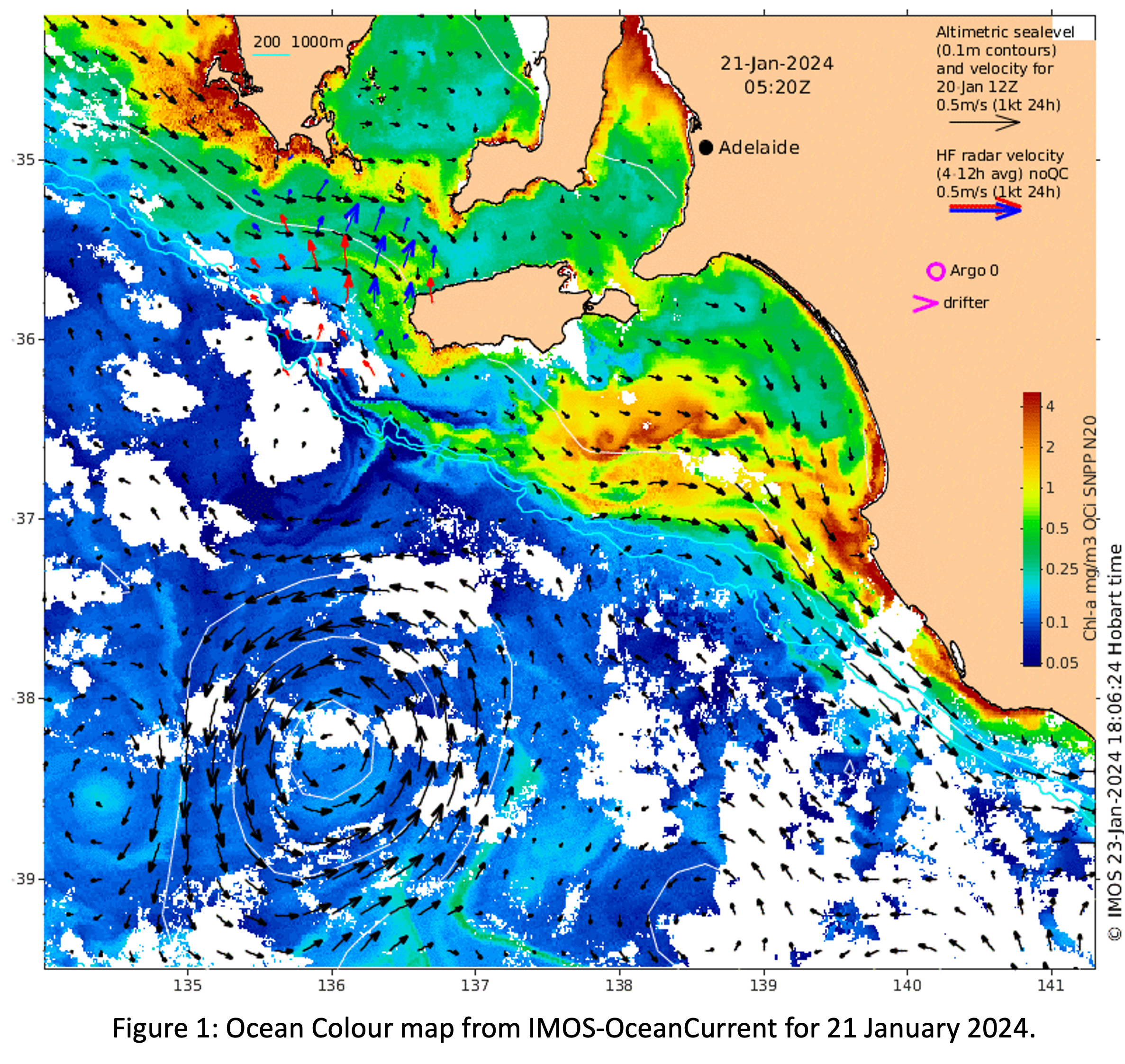
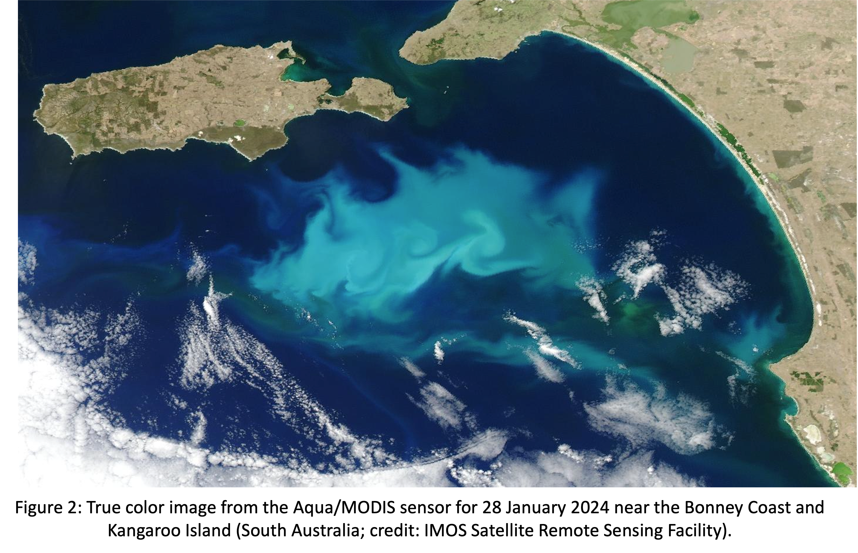
 Intense south-easterly storms have recently hit South Australia’s coast, causing strong upwelling events along the Bonney coast.
 We’ll keep our eyes out for the beautiful ocean colour satellite imagery we’ll see as a result.
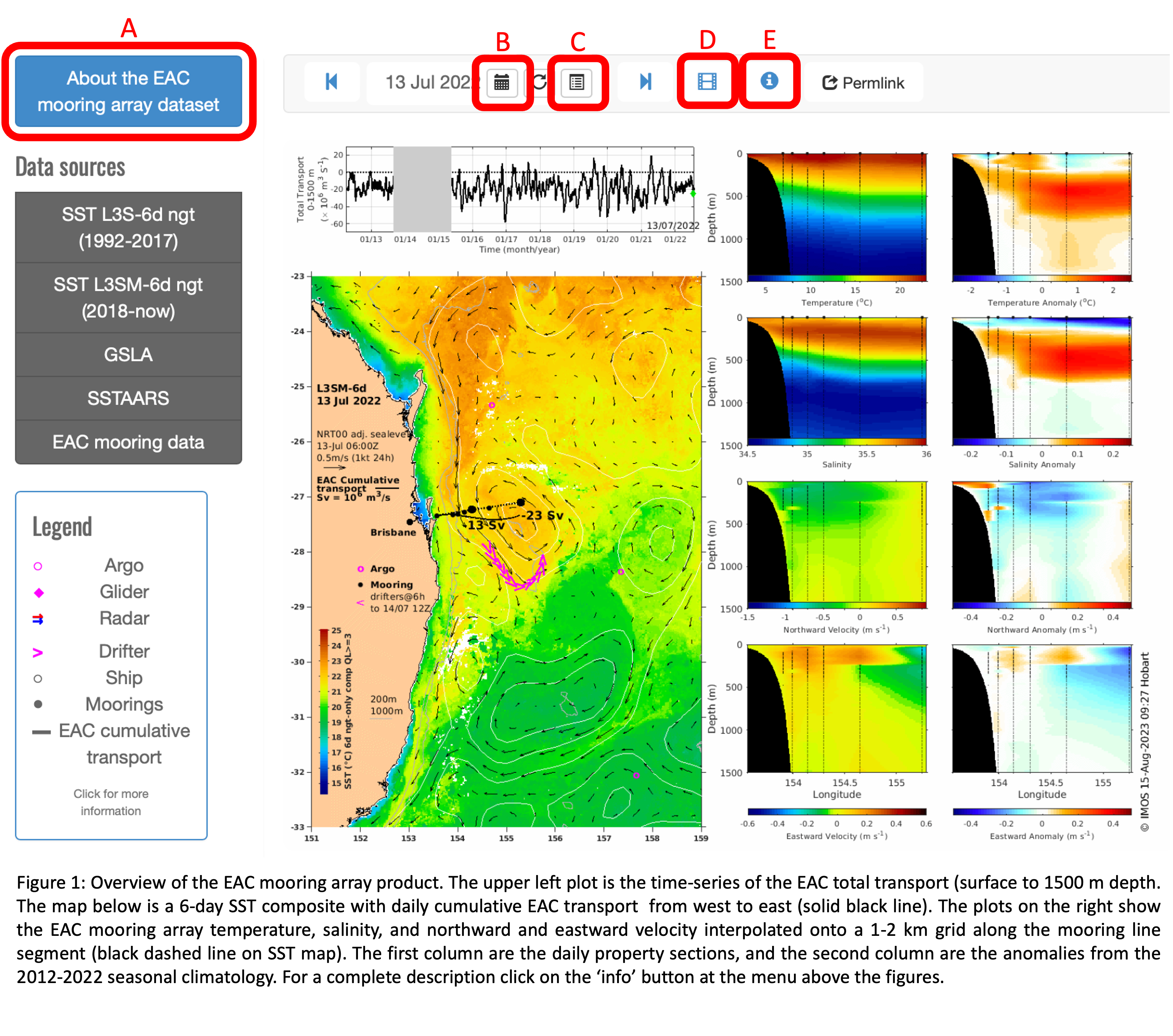
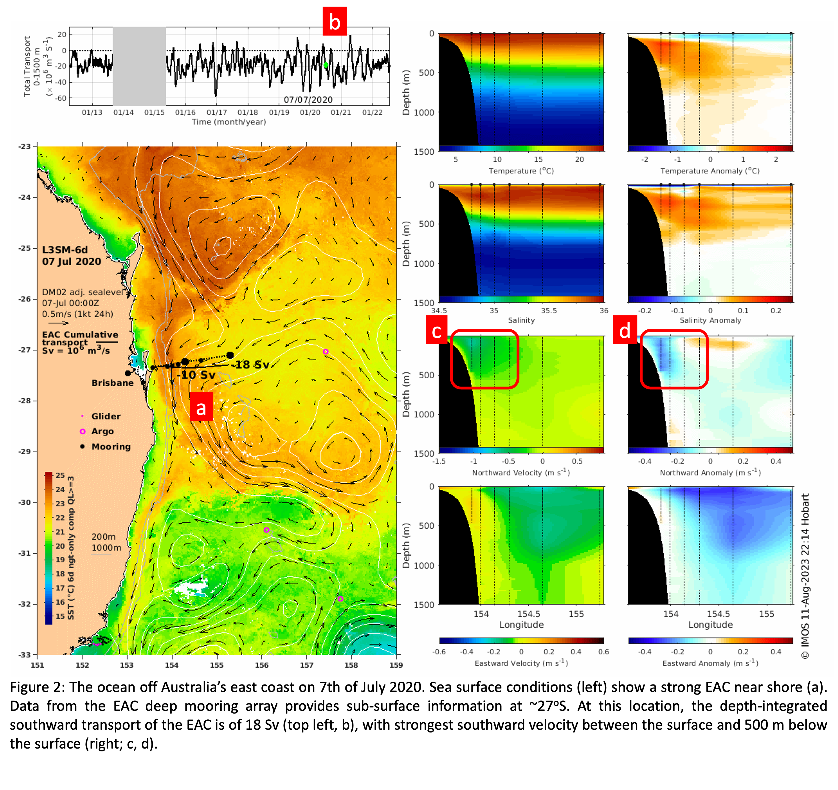 Looking at a particular day,
  Slack tide is when the tidal current turns from flooding to ebbing, or vice versa. If you need to conduct an operation during the period of weakest tidal current, this is when to do it. But published predictions of slack tide timings are very few, and there is no universal rule of thumb relating the timing of slack tide to the timing of high or low tide. For the case of a narrow strait leading into a large bay, slack tide in the strait occurs close to the times of high and low tide within the bay. In many places, however, it is far less clear, and slack tide occurs at different times in nearby places. In Clarence Strait (between Darwin and Melville Island), for example, slack tide is half way between high and low tide at Darwin. Stepping through
  Next week is the Australian Marine Science Association conference at the Gold Coast (at 28ºS). Since there will be a special IMOS session, and an East Australian Current session, how could we pack our bags without checking the state of the EAC? But disappointingly, from a morning dip perspective, the news is not good: the water is presently 19.5°C, about 2º less than climatology, sitting somewhere in the
  Our chlorophyll-a images are back! (Sorry about the outage.) To celebrate, let's contemplate one of the many riddles of Australian oceanography: what's the biggest difference between chlorophyll-a imagery of west coast and east coast eddies?
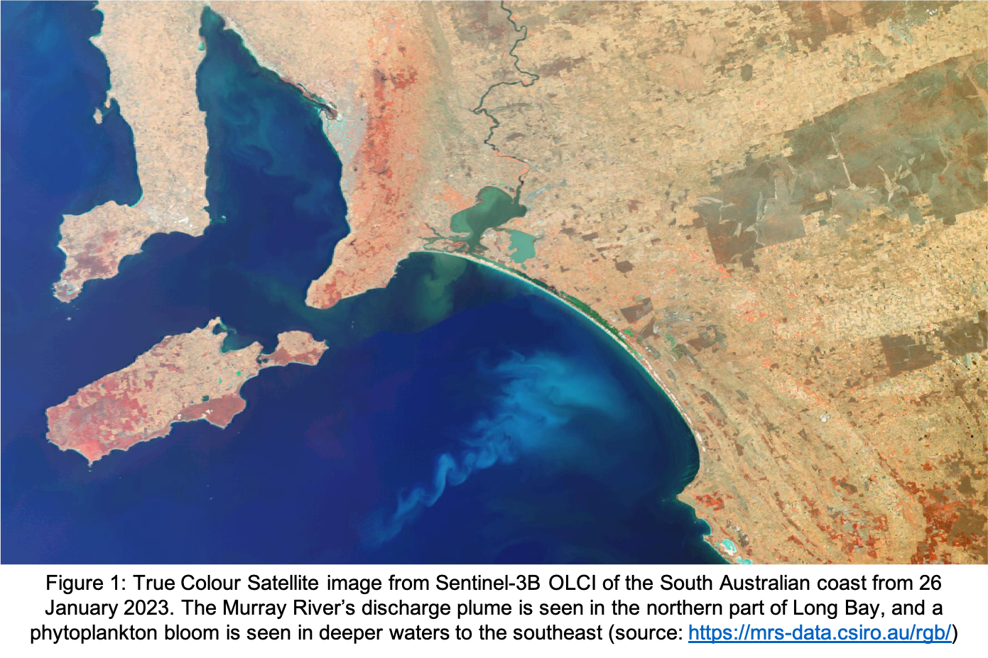
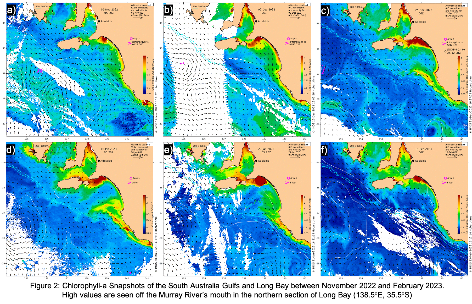
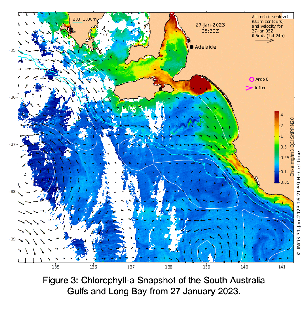
 There looks to be only one region between Sydney and Hobart this year where it is clear that navigators might like to factor ocean currents into their race strategy, and that's the far south of NSW, between about 36.5S and 37.5S.
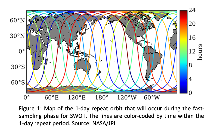
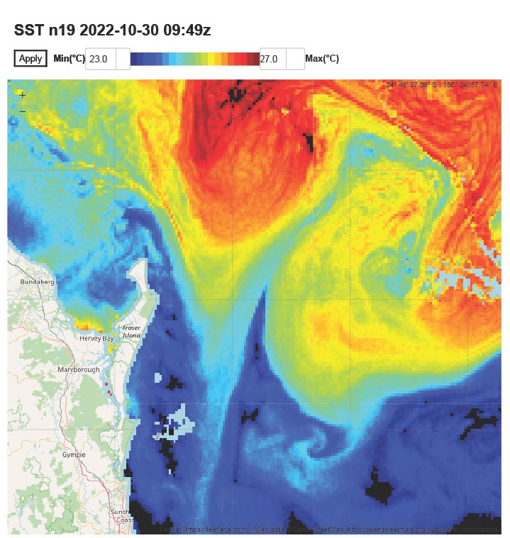 When looking at our maps of SST, do you ever wish you could zoom in or out to show whatever region you like, or adjust the temperature scale to enhance a particular feature? Well, now you can. We call it MyOceanCurrent, because you're in control. Access is via the green button on our landing page. Click Help if you need it. If you create a (free) MyOceanCurrent account you will get access to more viewing tools, and your settings will be remembered. Our example image zooming in near Fraser Island where a cyclonic eddy is interacting with the East Australian current shows some striking 'woodgrain' features in the warm waters aligned with the flow.


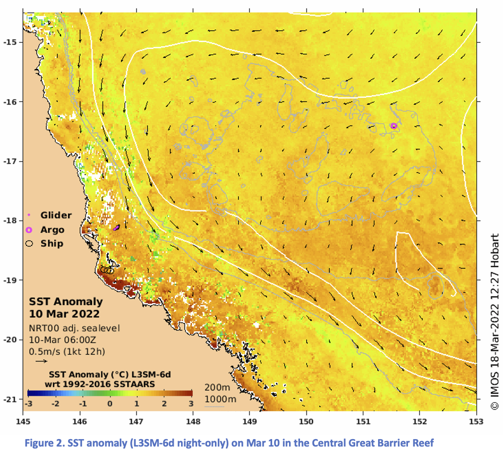
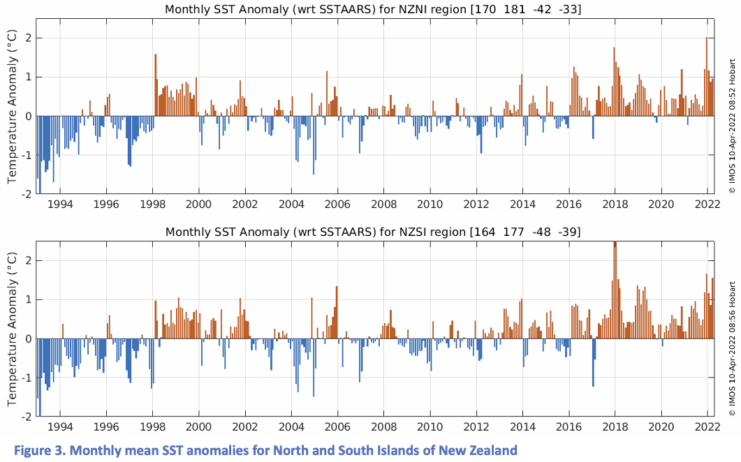
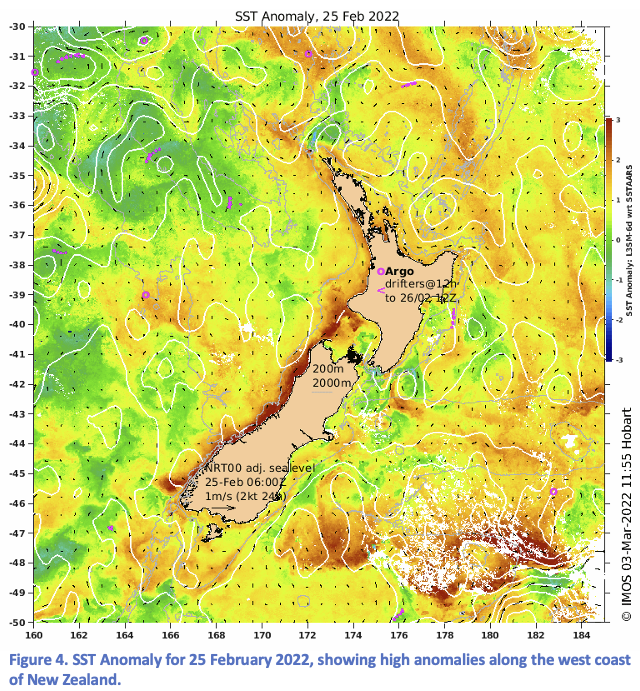

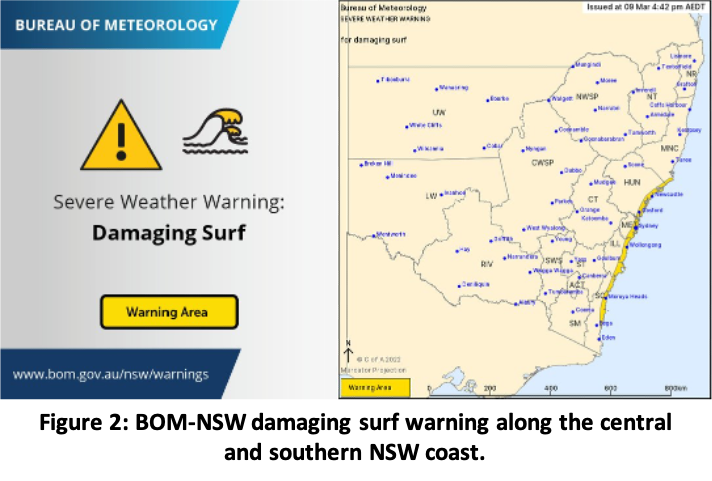
 This is the question that springs to mind whenever you see that the temperature, sea level, or other quantity is different from its 'normal' value. For some time now, we have made it easy for you to see how anomalous SST values are, by showing the anomalies in centile form. As of today, we are doing the same with the adjusted sea level anomaly (ASLA). A reminder of our intention to do this came on 12 October 2021 when we noticed that the ASLA over the shelf in the Great Australian Bight was very high (because of the strong south-westerly winds associated with a deep low centred that day near 42S 130E). By selecting 'Centiles' from the dropdown menu for Australian-region maps of ASLA, you can now see that the coastal sea level that day was indeed comparable with the highest few percent of all co-located anomalies in our archive of daily maps.
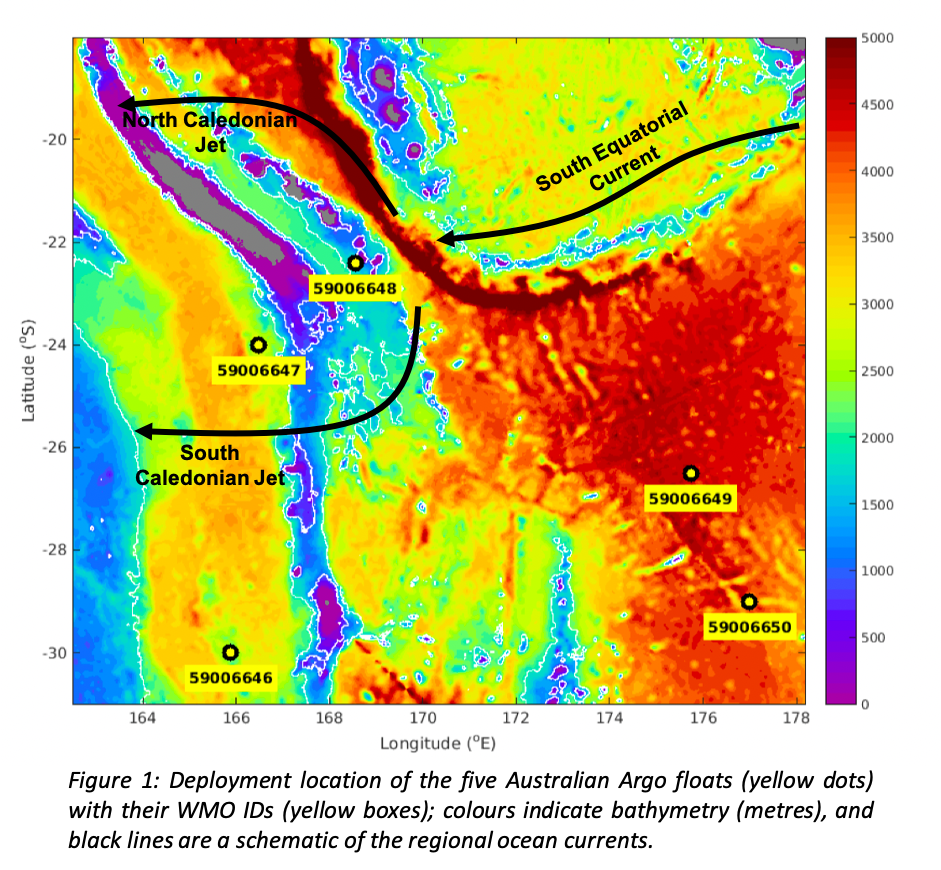
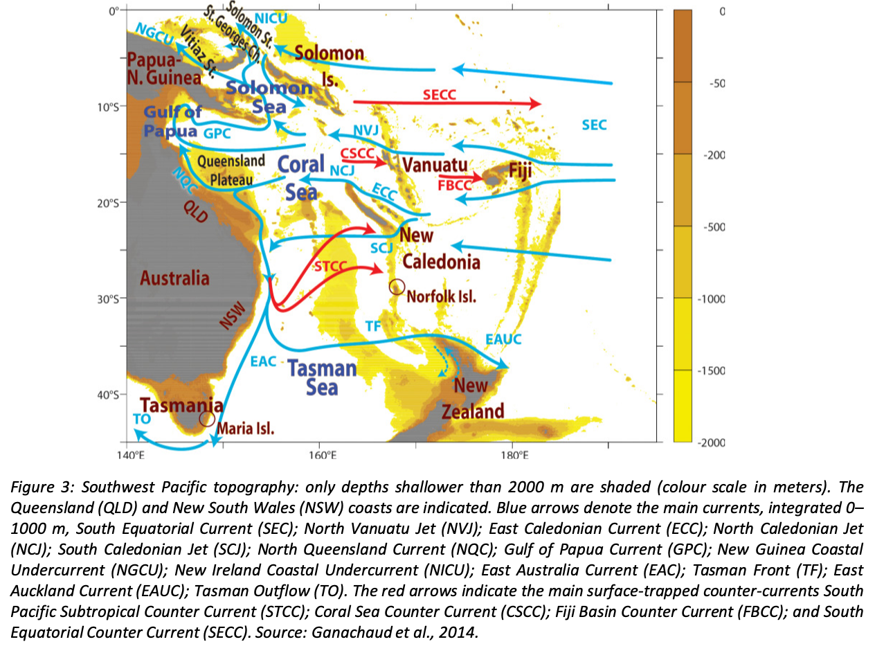
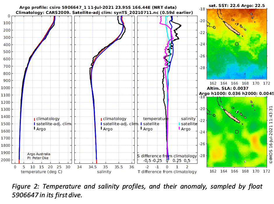
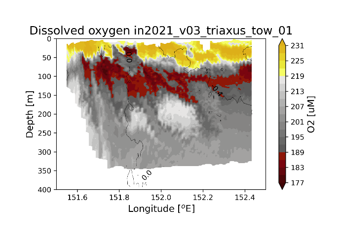

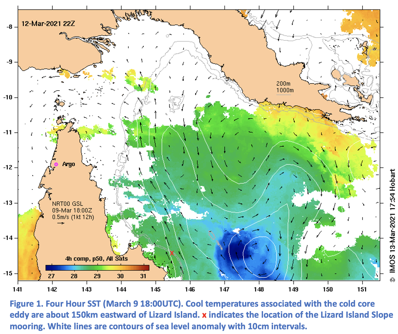
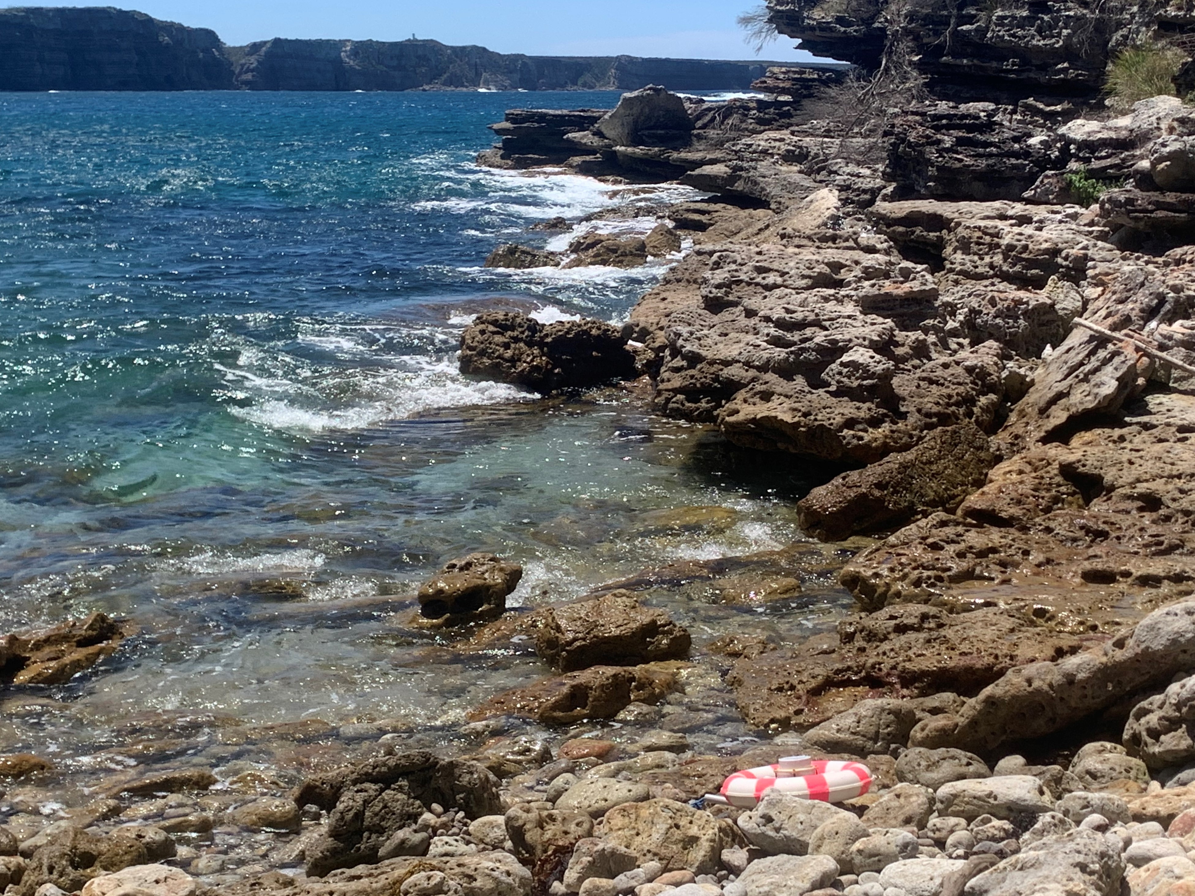
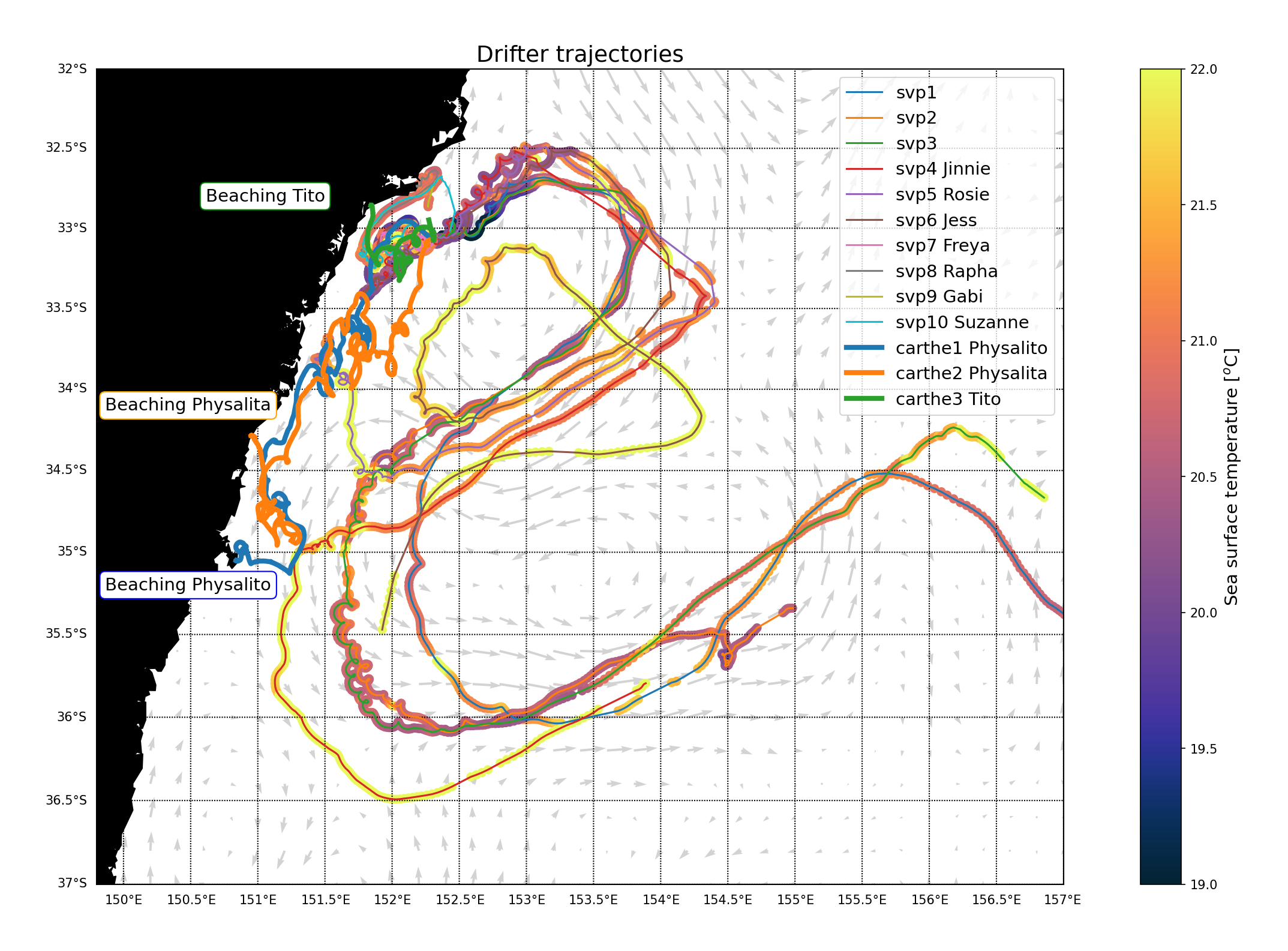


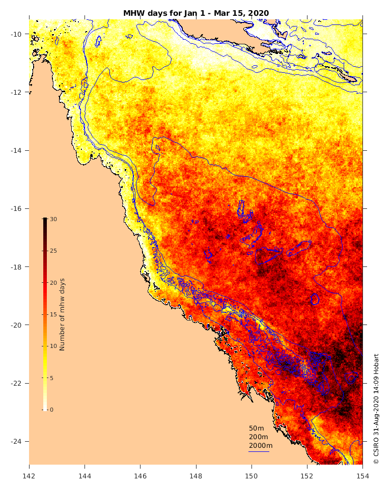
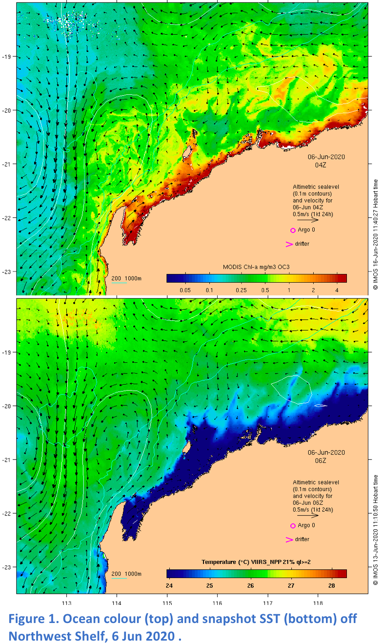 There has been no MODIS Aqua Ocean Colour data since August 16. Communication with the satellite is the issue, otherwise the satellite and sensor seem to be operating as normal. NASA are still investigating the situation and will be attempting a reboot over the coming days. It’s hopeful transmissions will resume shortly.
 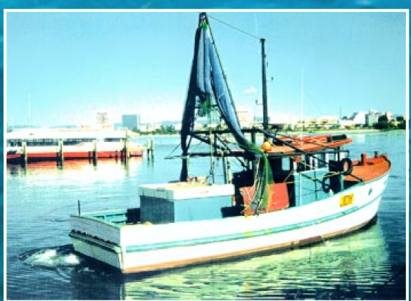 Late on New Year’s Eve 1995 Mark Beveridge’s prawn trawler, the Jay Dee, was hit by a large ship 16 miles or so out from Southport on the Gold Coast. Mark was the only person on board. His boat sank quickly. He had no food, no water and was dressed in singlet and shorts. He spent the next 40 hours drifting southward with a small life raft and an icebox. He knew that he had to get to shore before he reached Cape Byron or he would be swept out to sea by the East Australian Current. EAC pioneering observer George Cresswell assisted the Australian Transport Safety Bureau's 1996 investigation into the events surrounding the sinking of the Jay Dee. George has now re-examined the question of how Mark was so fortunate to survive. Anyone with an interest in survival at sea will find Mark's account of his tribulation, and George's contextualization of it, something to ponder deeply.
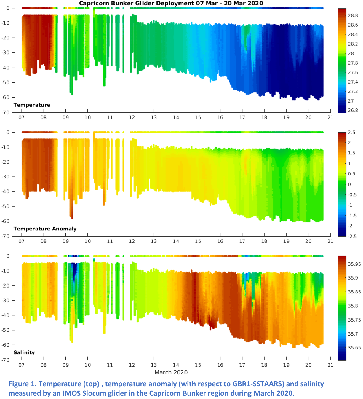
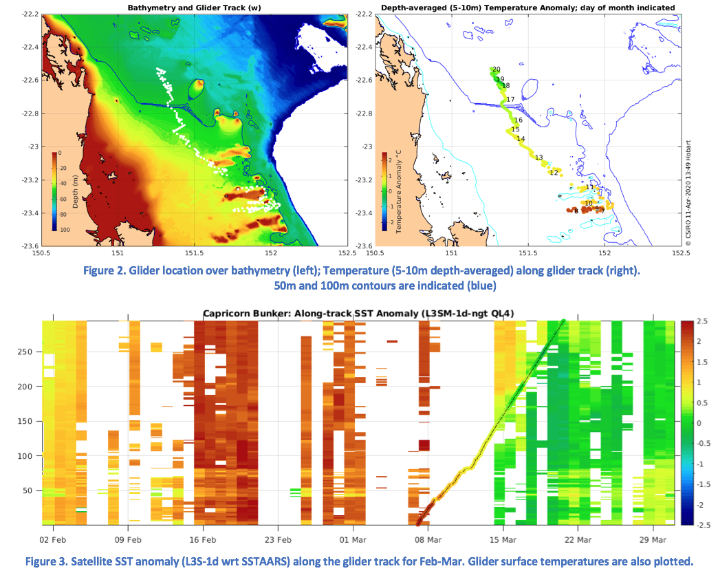
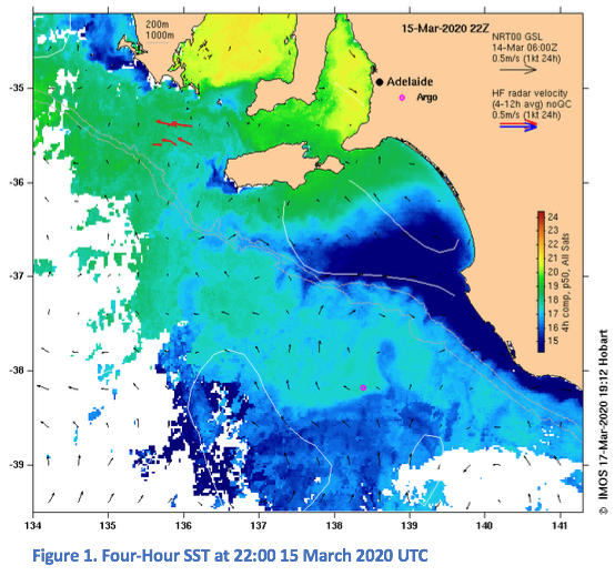

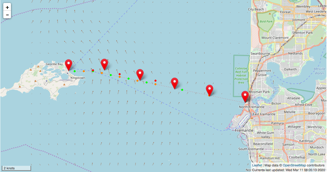
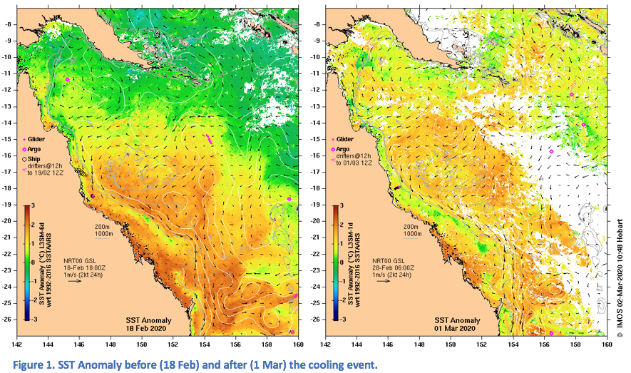
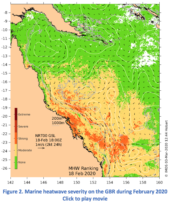
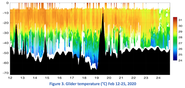
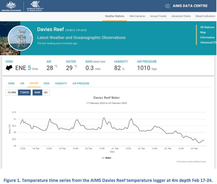 Observations of water temperature from the AIMS Davies Reef station, 18.8°S 147.6°E (Figure 1), show temperatures have dropped by well over 1°C since Friday. This cooling represents a significant relief from the previous 10 days of heatwave conditions and appears to be widespread with similar cooling at Heron island (23.5°S) and Yongala (19°S). From the temperature time series we can see that the daily pulse of diurnal heating has stopped thanks to the cloud and rain that has developed along the Queensland coast, covering much of the GBR (Figure 2).
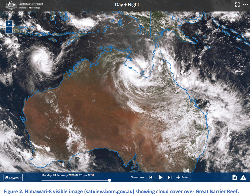 How long can this cooling last? The onshore winds responsible for bringing the moist air from the Coral Sea to feed the clouds are driven by the pressure gradient between the low trough in the north (including TC Esther in the Gulf) and the high pressure system in the Tasman Sea. The forecast is for this pressure gradient to dissipate on Tuesday but that rain may persist for the next few days after that.
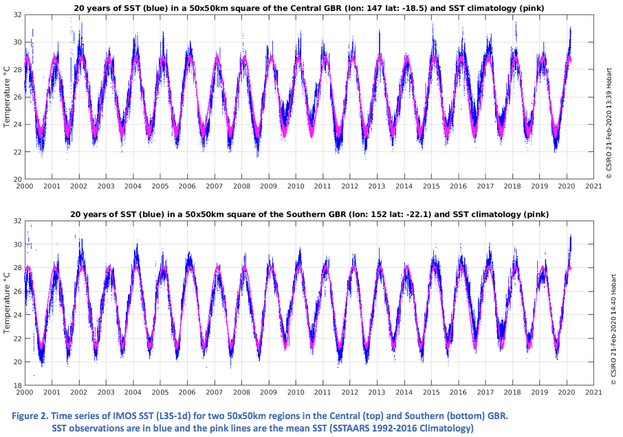
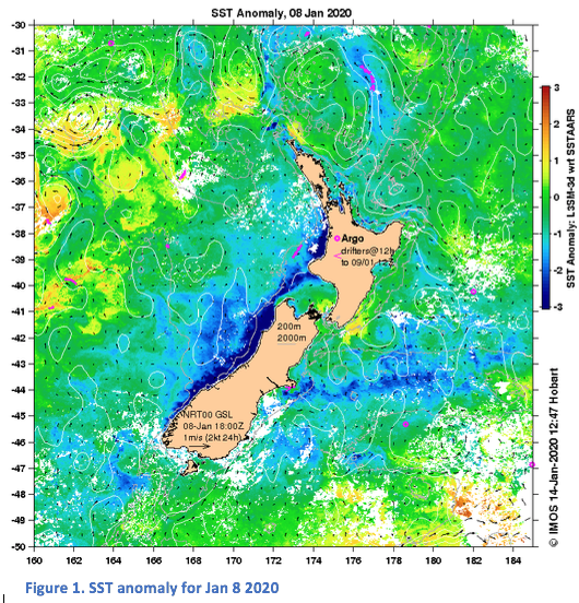
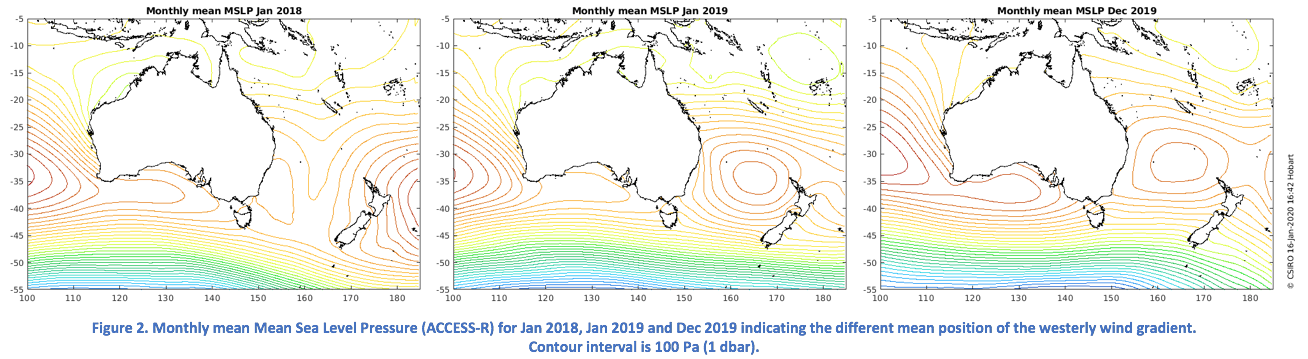
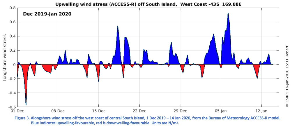
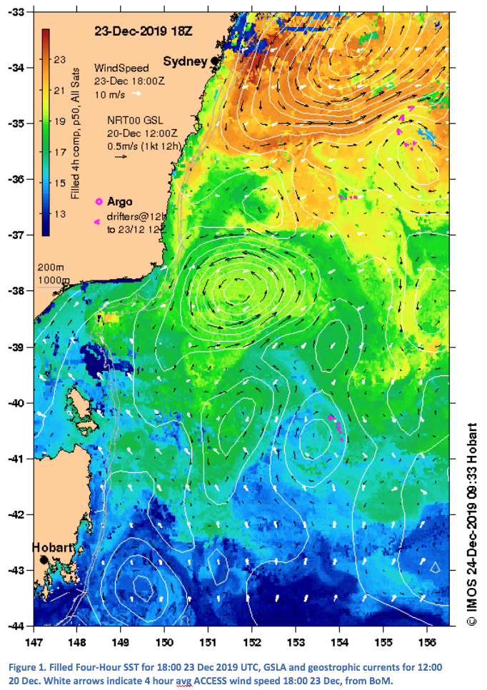
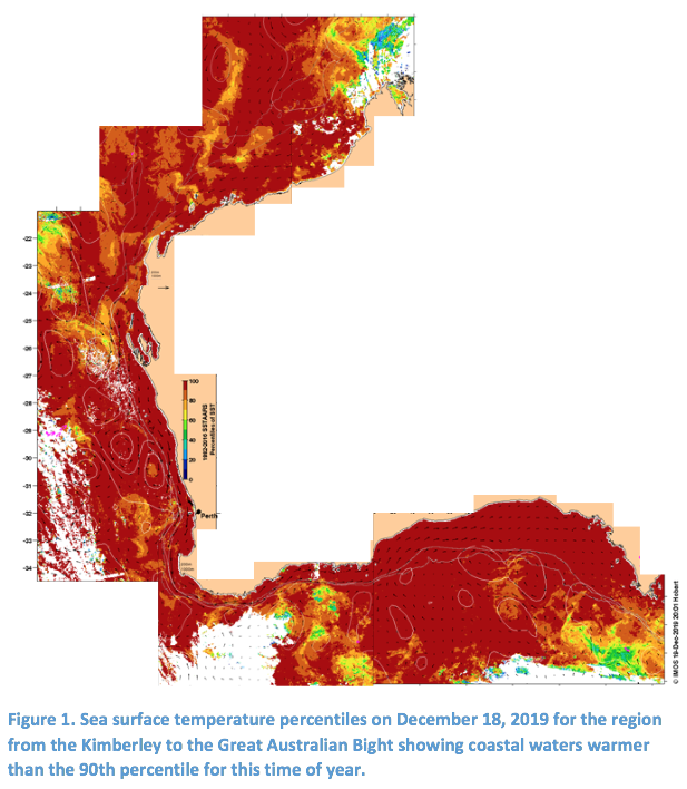
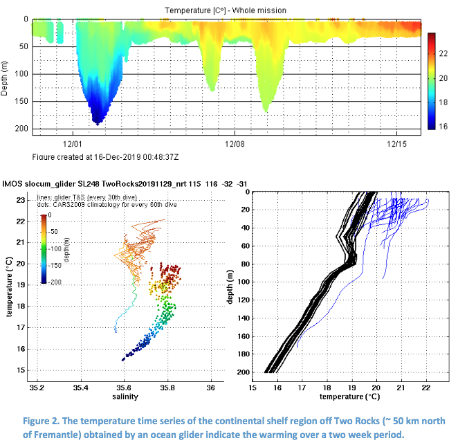
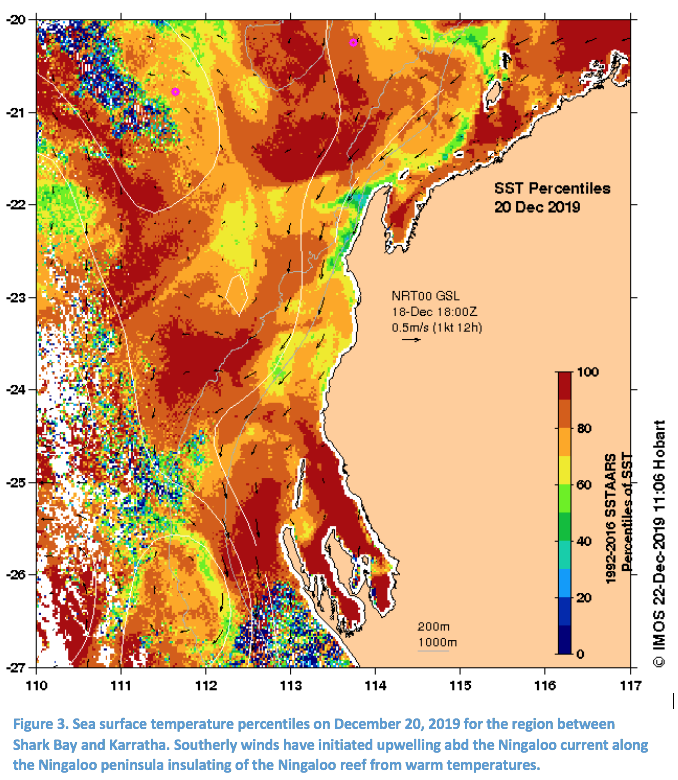
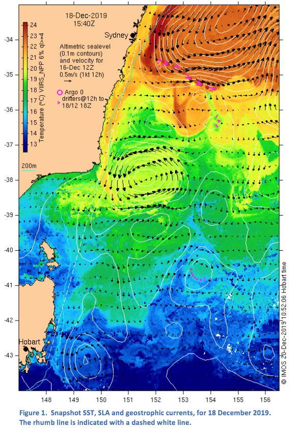
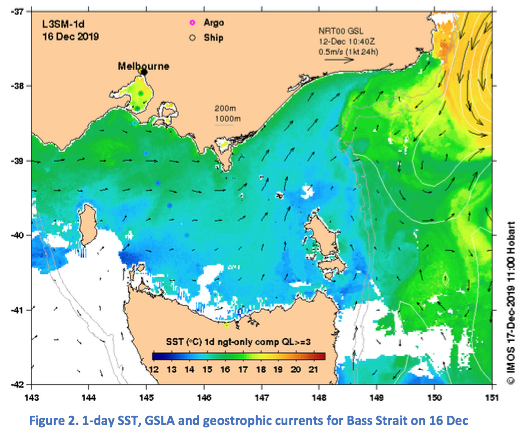
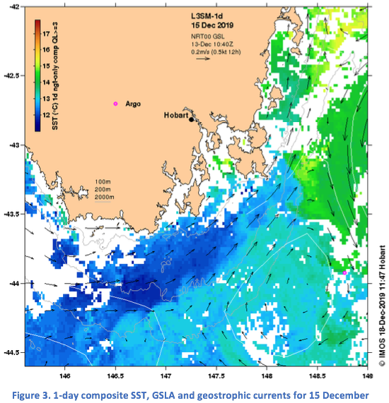

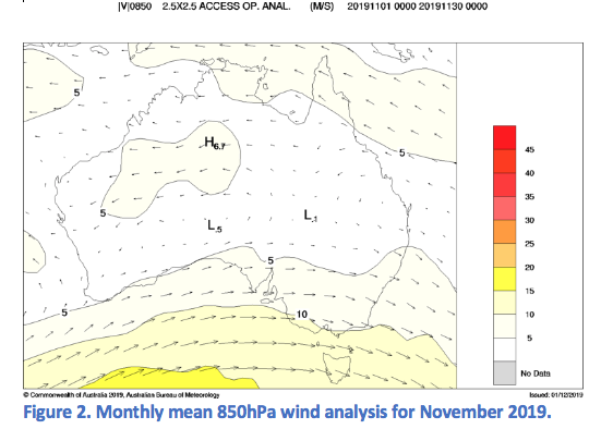
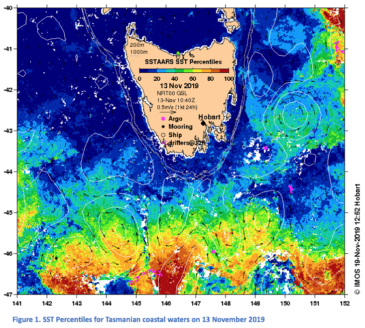
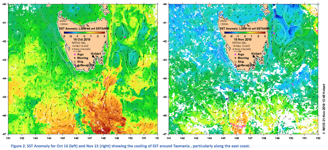


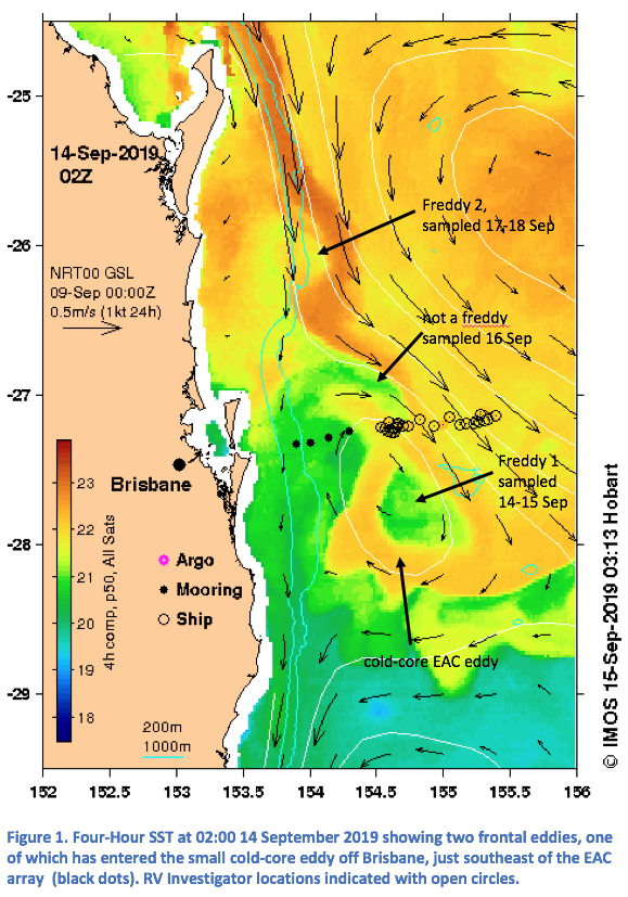
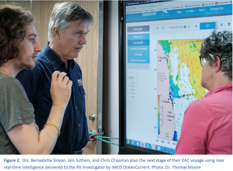

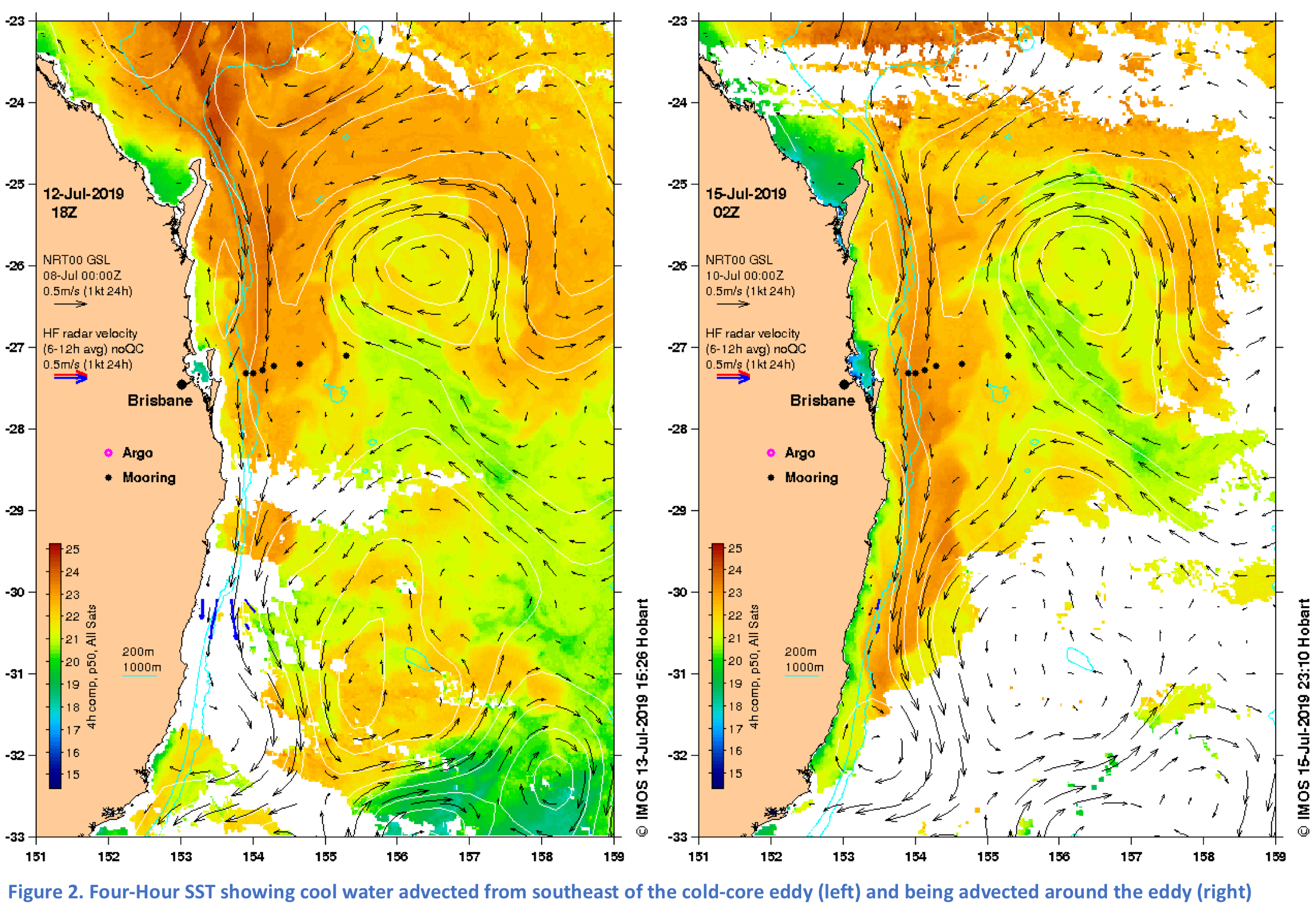
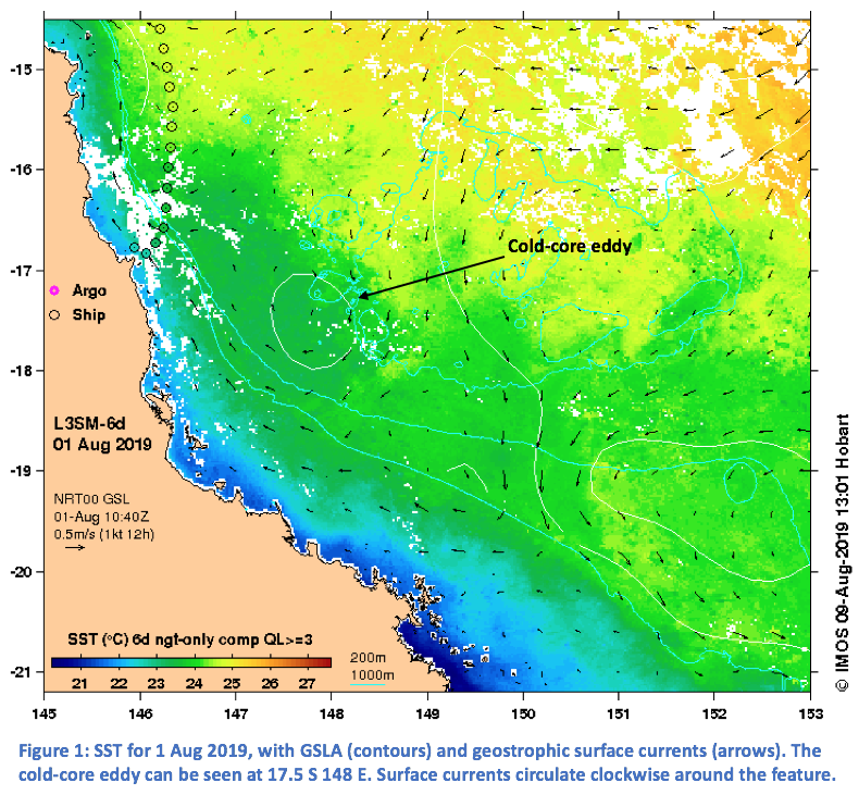
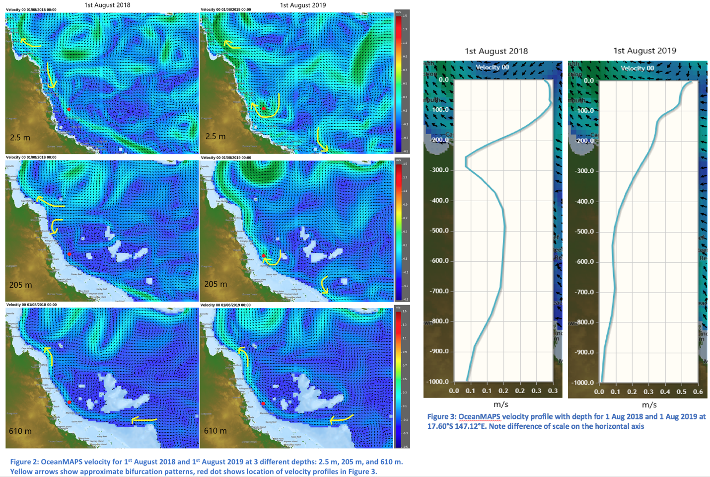
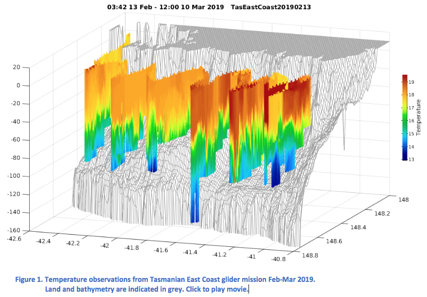

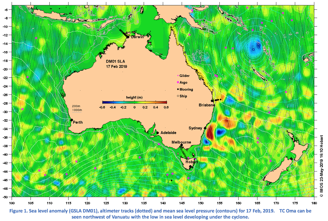
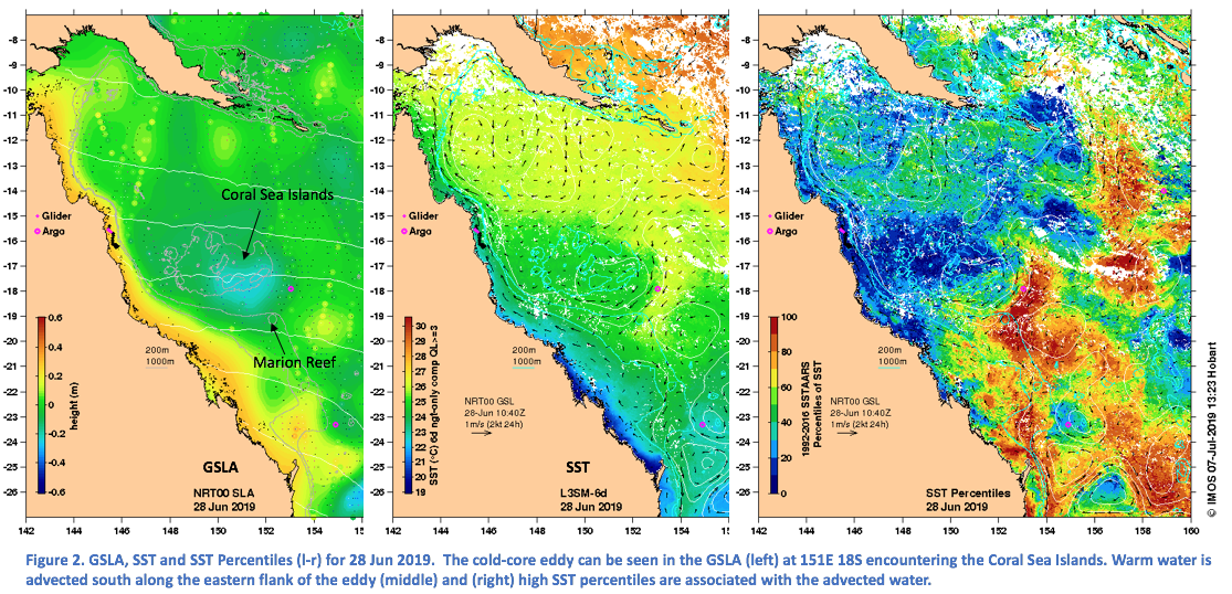


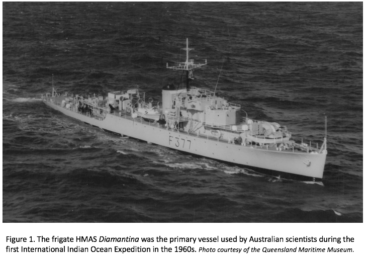

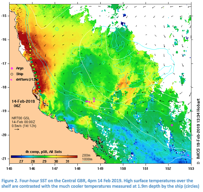
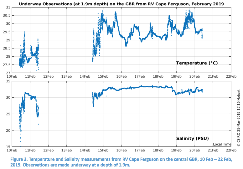
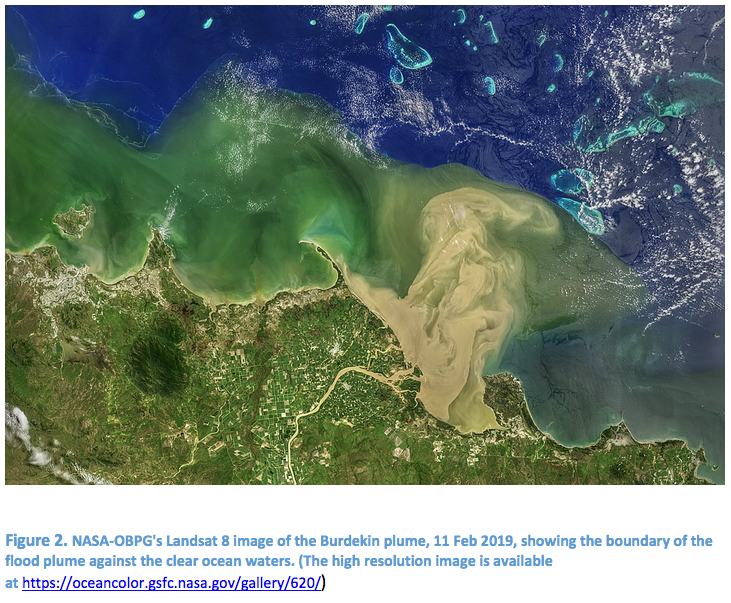
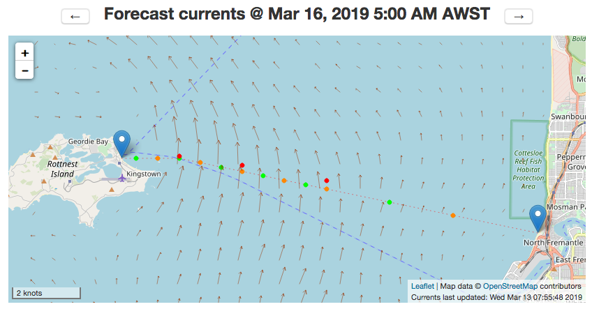

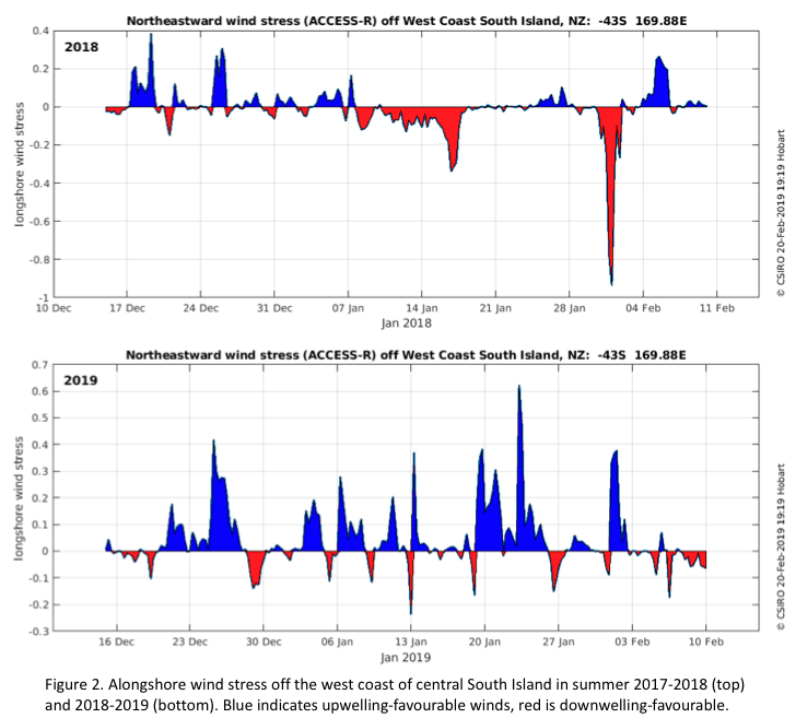
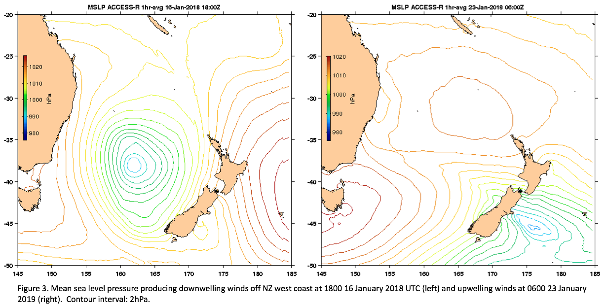
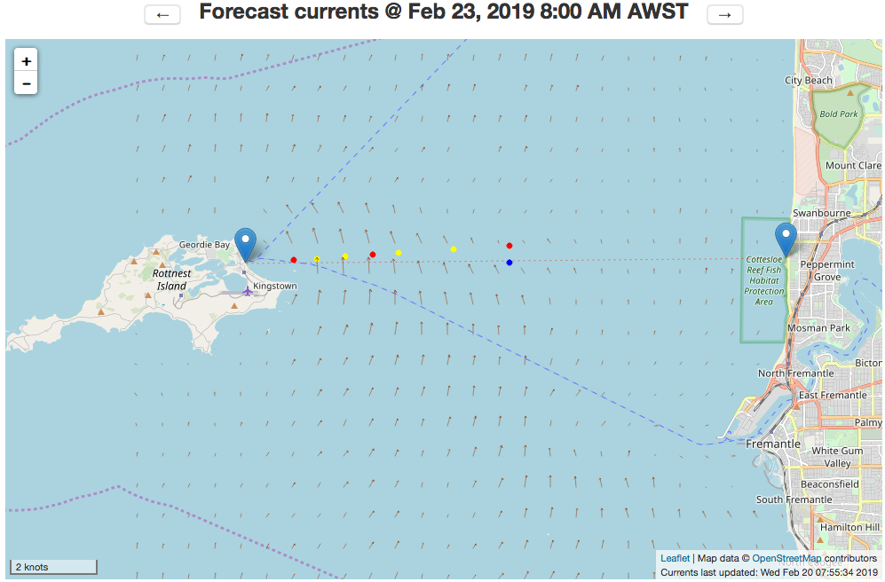

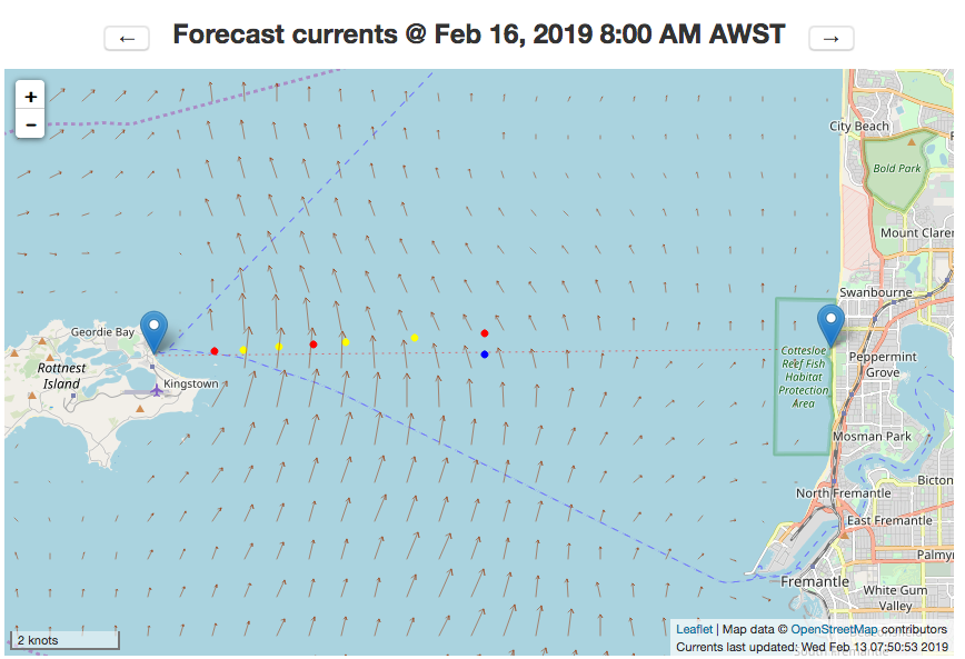
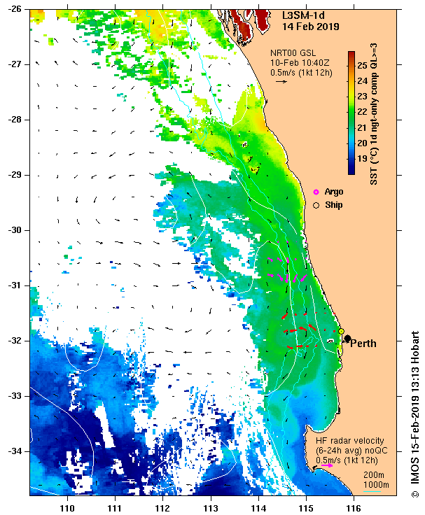
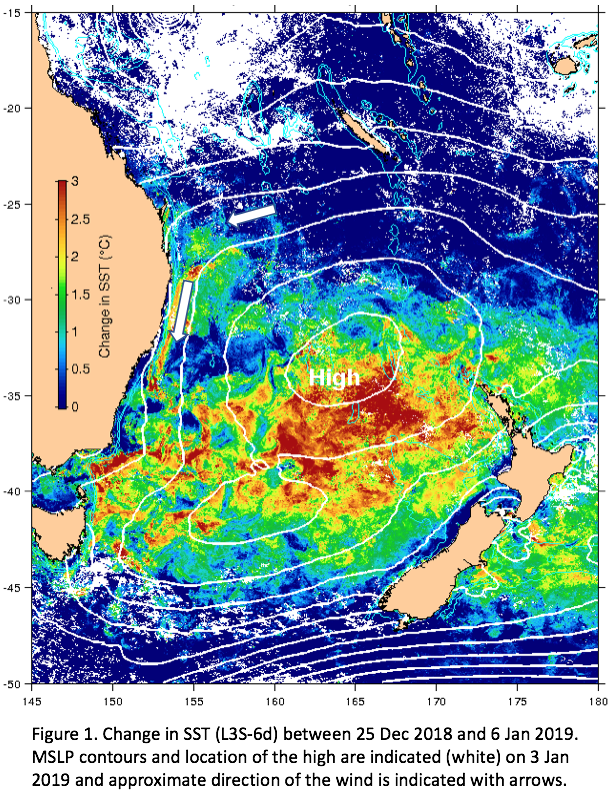
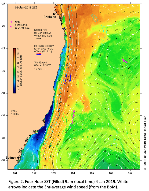
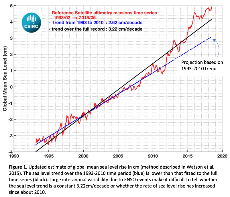
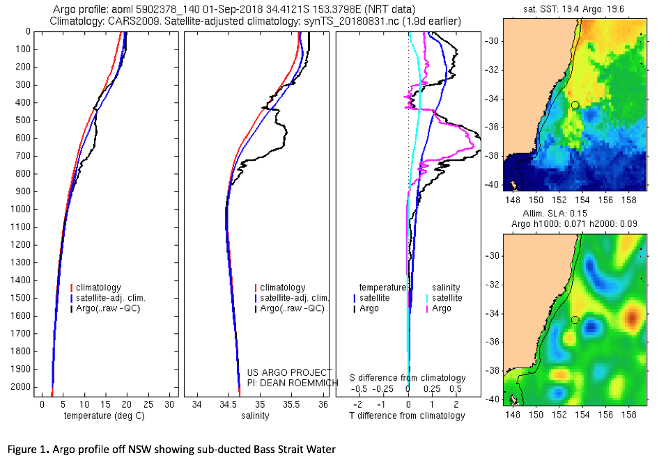 An Argo float (WMO # 5902378; deployed in 2014) that drifted near the continental shelf off central New South Wales on 12 August 2018, showed
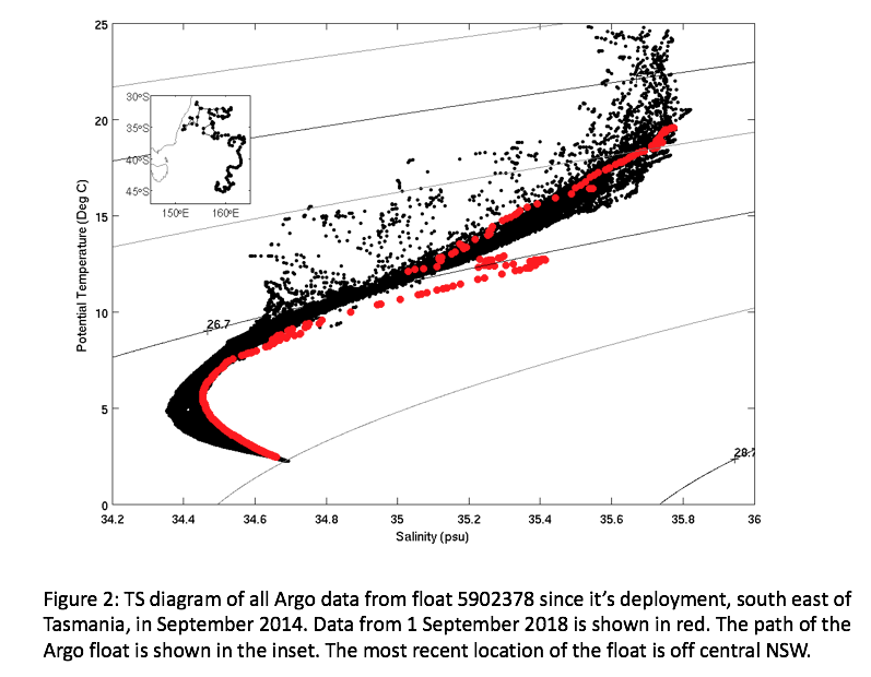

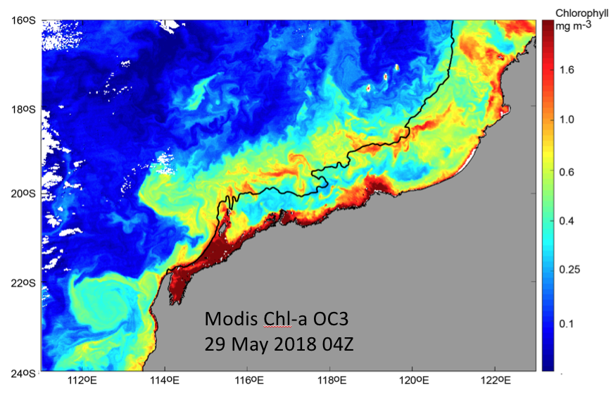 Ocean fronts, defined as regions of large horizontal gradients in water properties (temperature, salinity etc), are areas of high productivity globally. Recent satellite imagery from the north-west shelf indicates the existence of two types of fronts extending over 1000km from North-West Cape to Cape Leveque. The nearshore band of high chlorophyl is associated with a
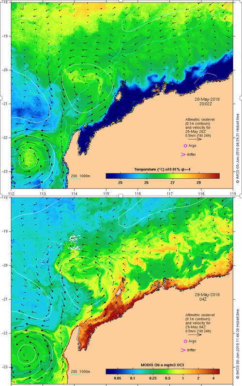
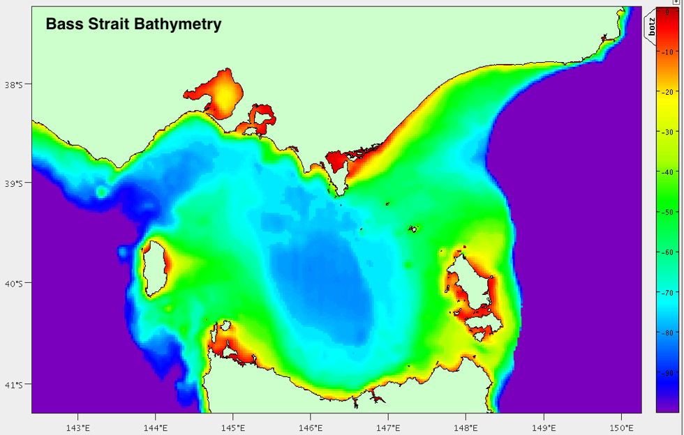

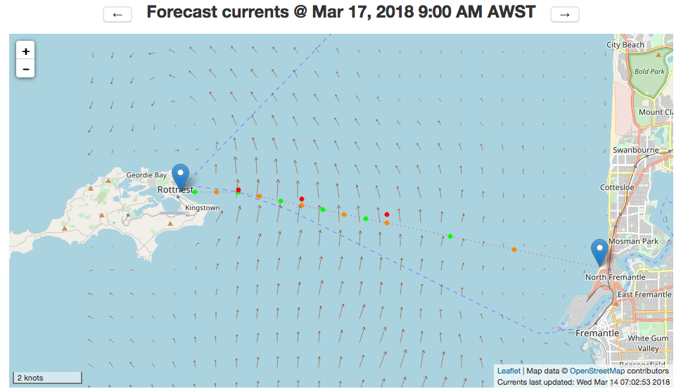
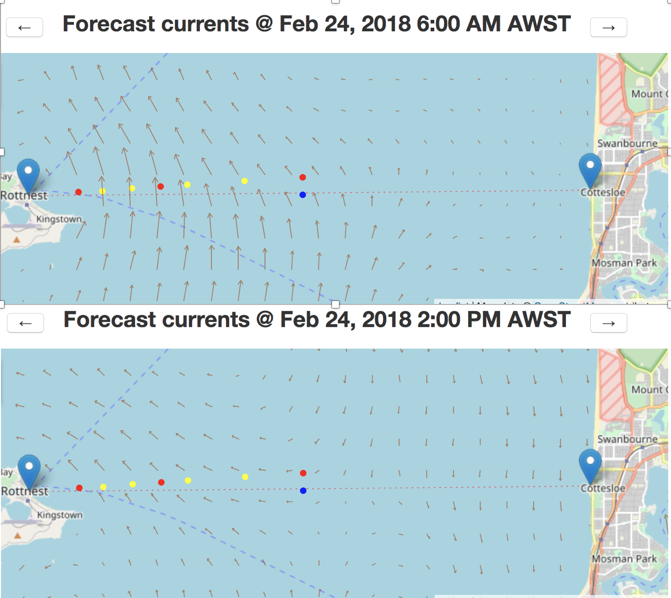
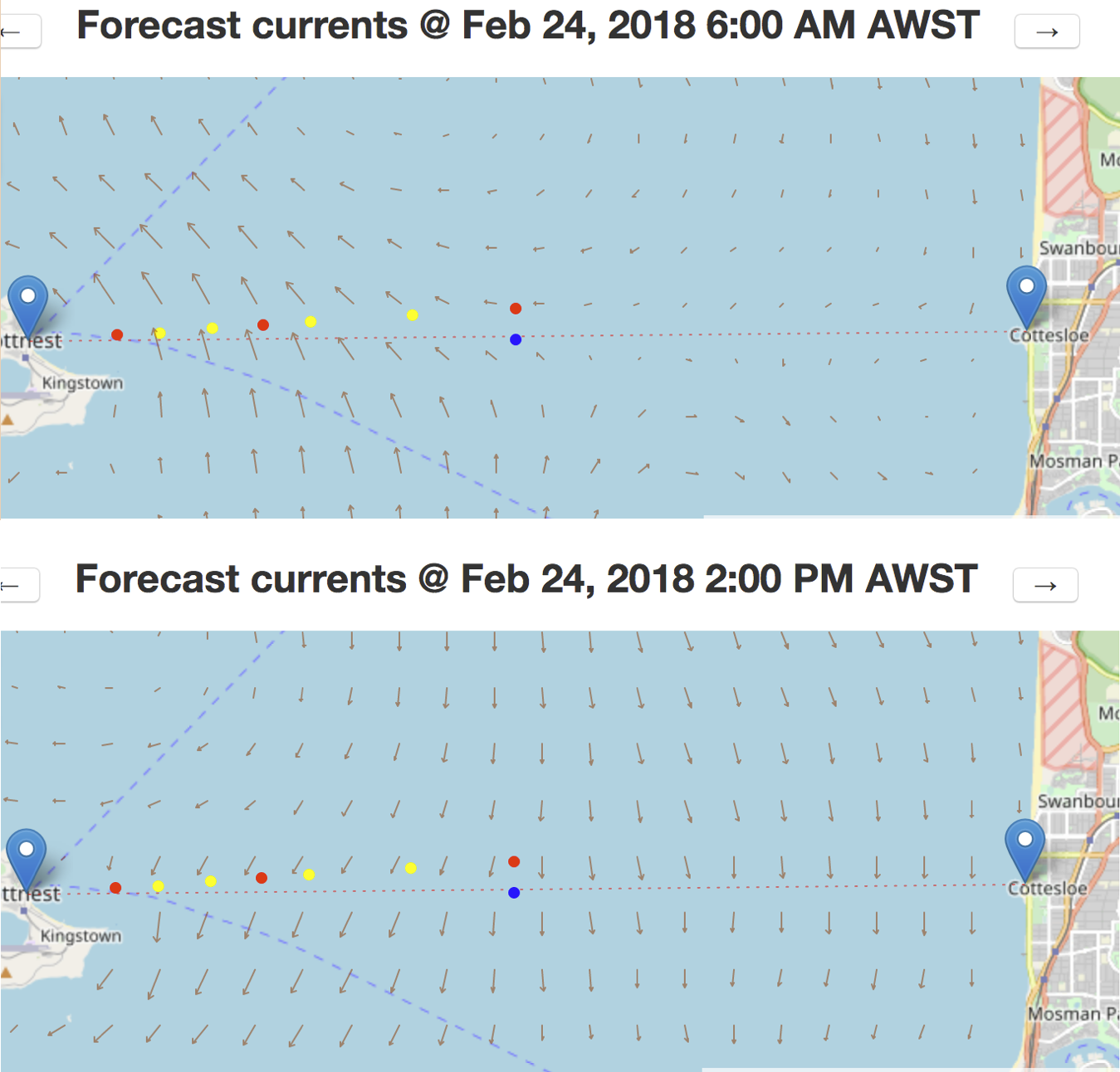
 Sea surface temperatures around Tasmania were


 We recently added the tracks of our well-equipped seals to our archive of high-res satellite imagery (chlorophyll, SST and surface current). A 2014 trip by a male New Zealand Fur Seal from Montague Island to Jervis Bay – the long way - is particularly intriguing. The image at right shows the final 2 days of his trip around a warm-core, low surface chlorophyll eddy of the East Australian Current. His voyage started on 8 September and if you step through
 It has been over a month since the tropical leatherjacket species started washing up on the beaches of far-eastern Victoria.
 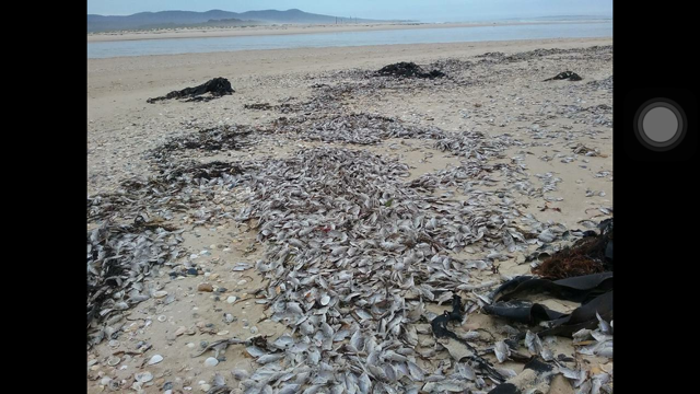 Thousands of dead fish have been washing up on the shores of far eastern Victoria and southern NSW. They started appearing on the beach in small numbers around March 11 but came in en masse in the last few weeks of March. Although most of the fish appear to be leatherjackets, there are also whiting, black sole, puffer fish, boxfish, sea urchins, flathead and even some penguins.
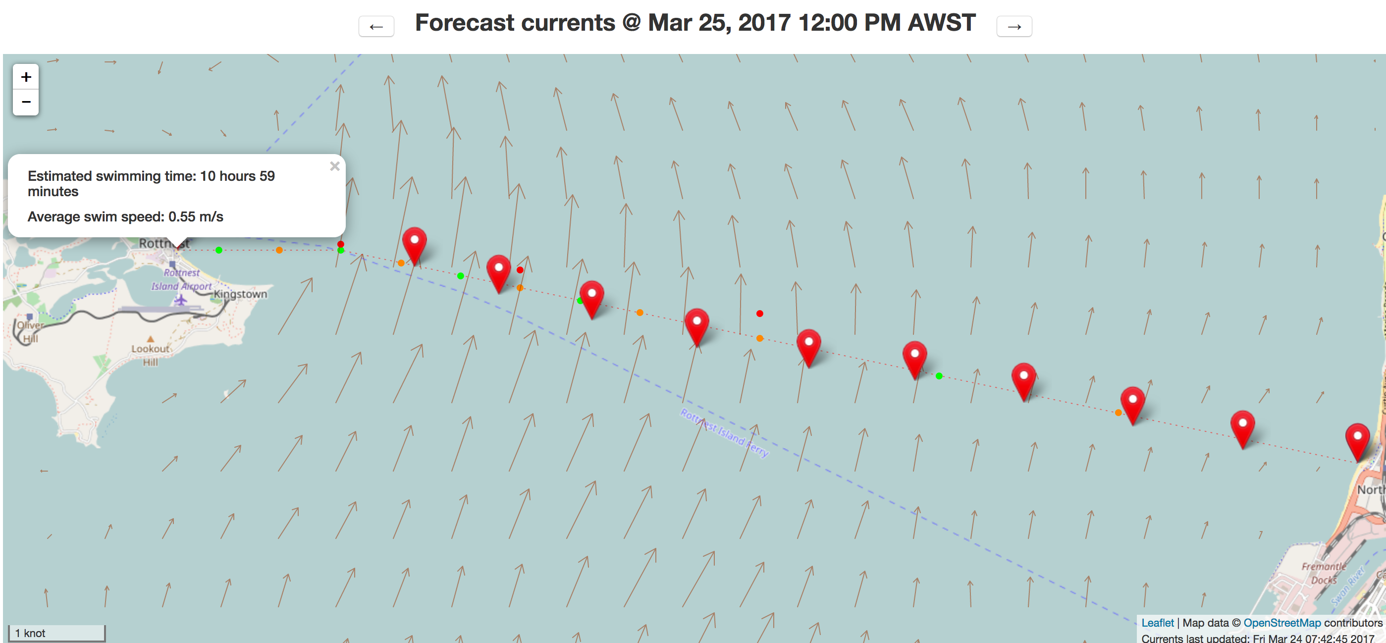
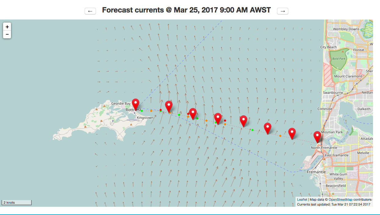
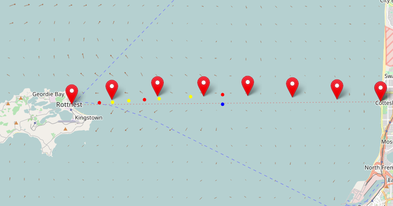


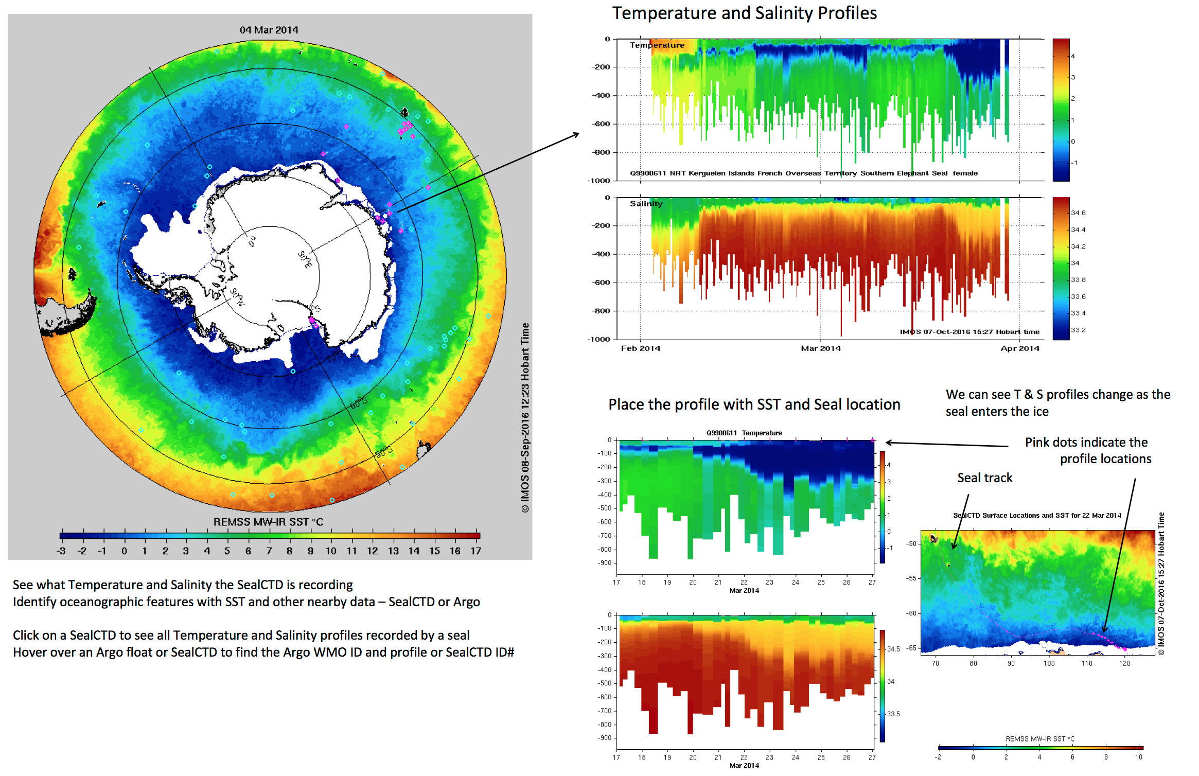
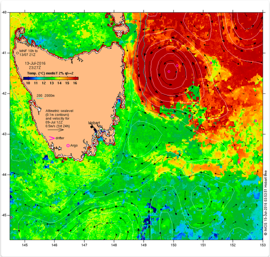
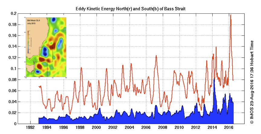
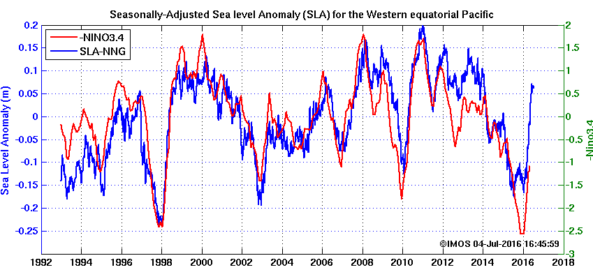

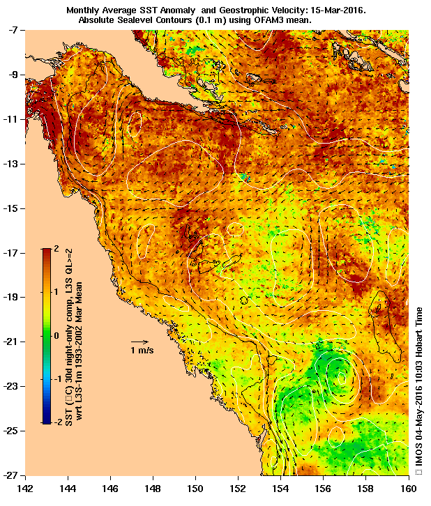
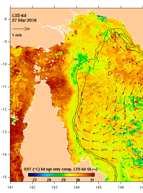
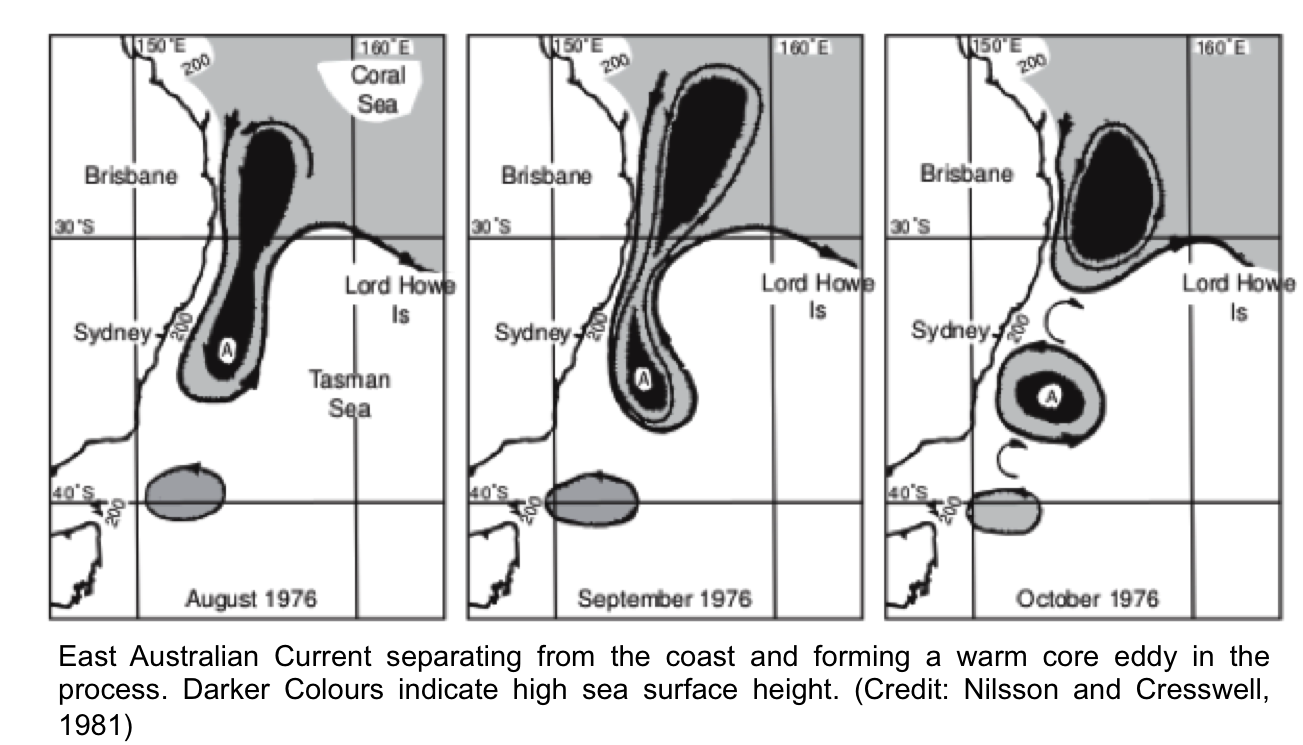
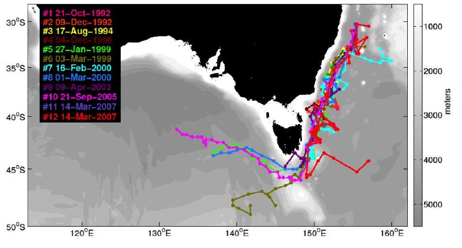
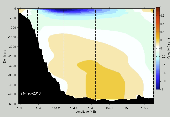 Ocean western boundary currents redistribute heat around the world and have a profound effect on the world’s climate.
The East Australian Current (EAC) is the major pole-ward flowing current of the South Pacific.
It provides the dominant mechanism for transporting heat from the equatorial Pacific to the cooler mid-latitudes.
Satellite observations show the spatial extent and variability at the surface but the subsurface velocities and properties can extend to
depths of thousands of meters and remain largely unknown.
Ocean western boundary currents redistribute heat around the world and have a profound effect on the world’s climate.
The East Australian Current (EAC) is the major pole-ward flowing current of the South Pacific.
It provides the dominant mechanism for transporting heat from the equatorial Pacific to the cooler mid-latitudes.
Satellite observations show the spatial extent and variability at the surface but the subsurface velocities and properties can extend to
depths of thousands of meters and remain largely unknown.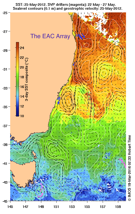
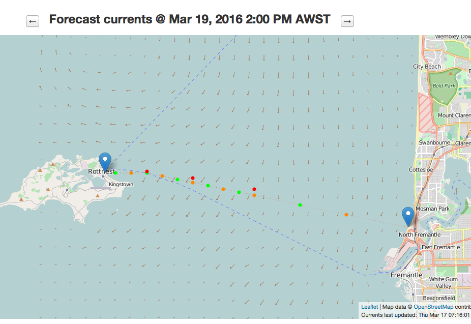

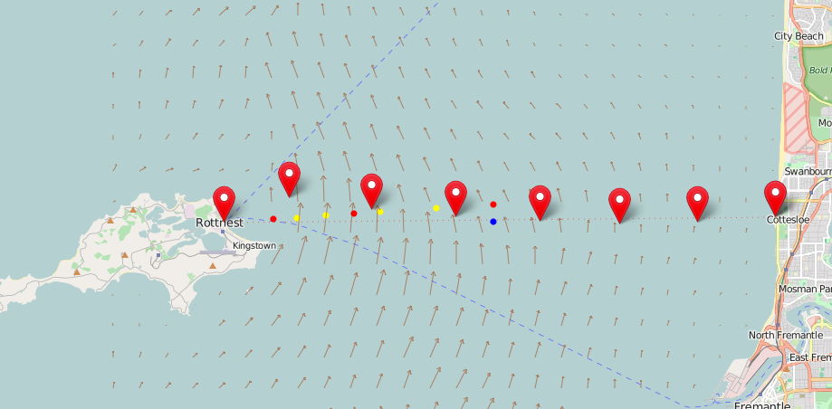
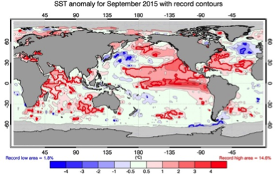
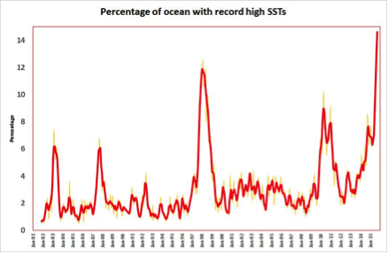
 There has been speculation in the media that the on-going sea-floor search for MH370 is being conducted in the wrong area. This speculation rests on modelling that suggested that the flaperon found on La Reunion on 29 July 2015 probably entered the ocean more than 1000km north of the present sea floor search area. This speculation is at odds with CSIRO, who concluded that the finding of the flaperon “did not cast doubt” on the sea-floor search area.
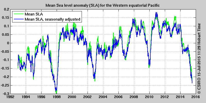
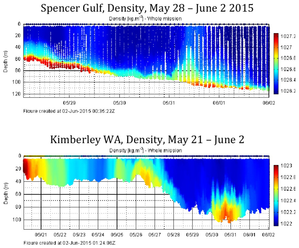
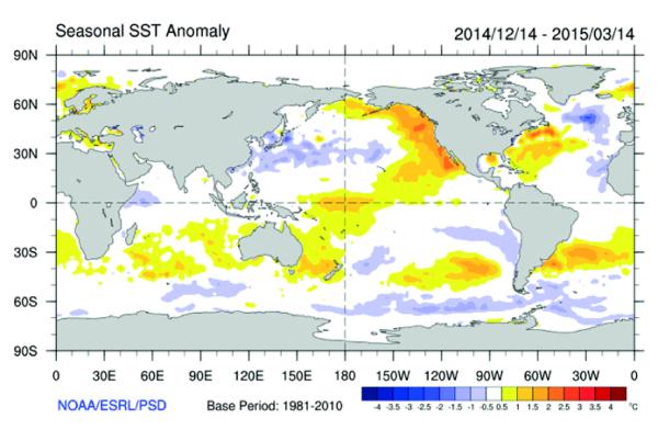
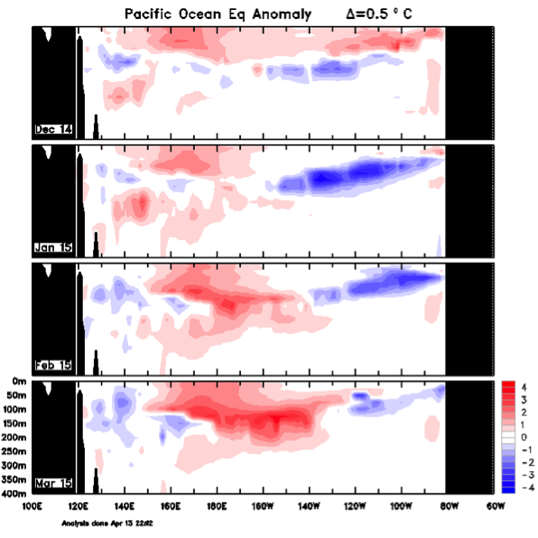
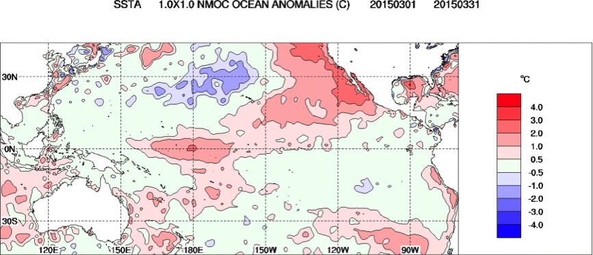
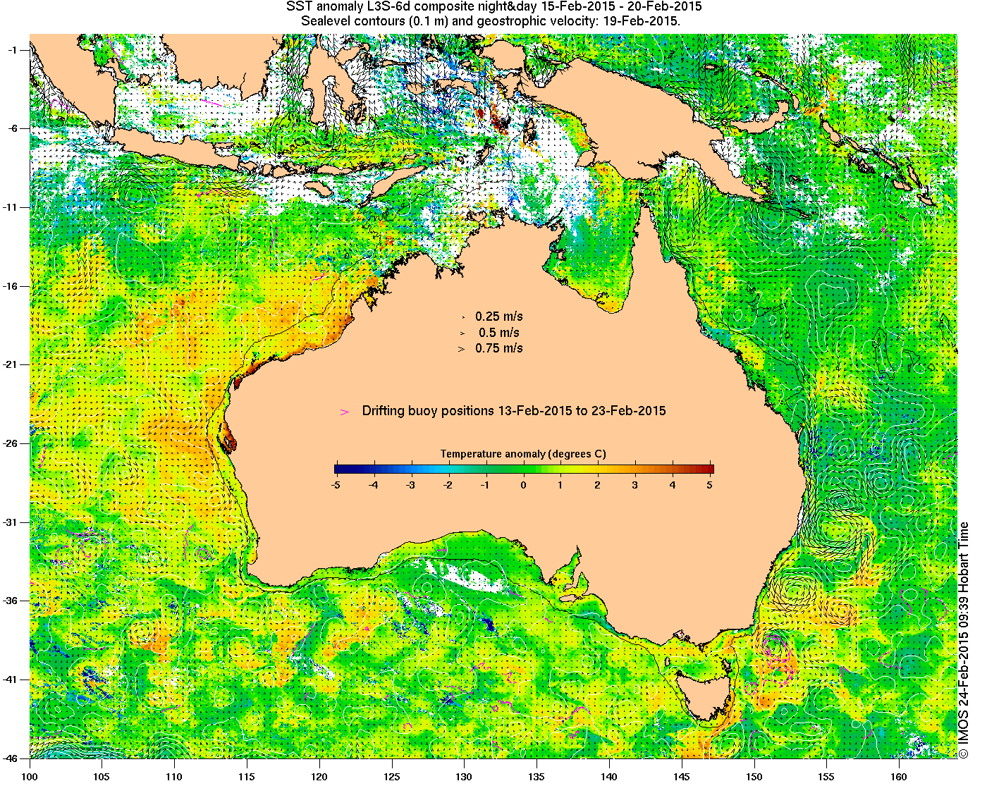
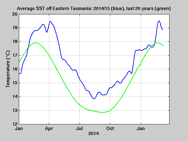

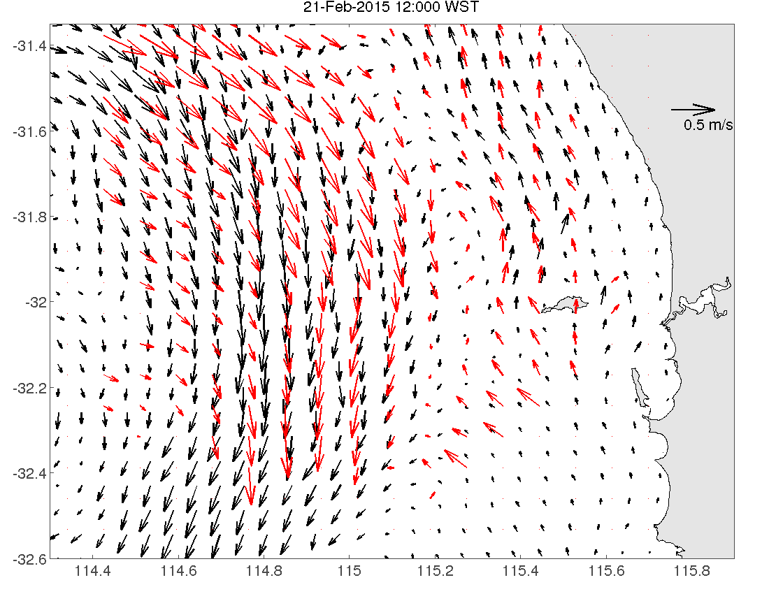
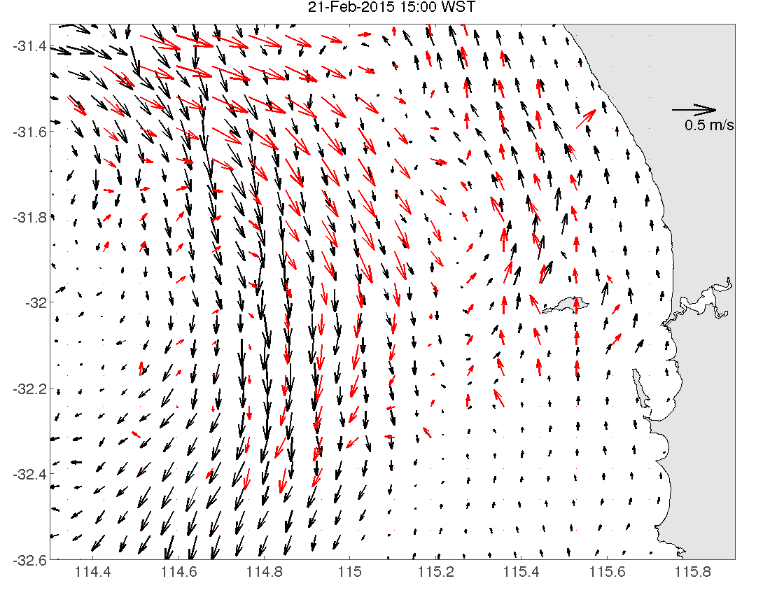
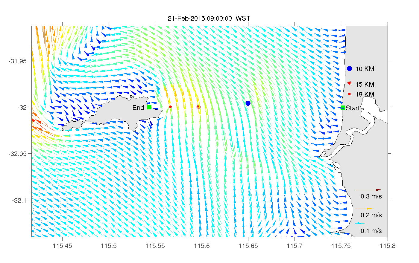

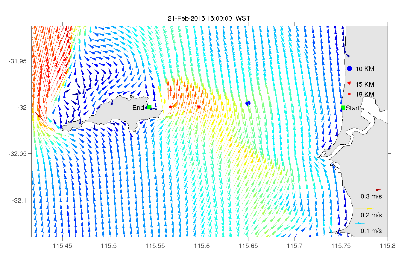