IMOS-OceanCurrent maps: What's shown?
The IMOS OceanCurrent maps are divided into three categories, according to their spatial scale: local regions, state regions, and the whole Australian region. These maps include various combinations of satellite-derived datasets and in-situ datasets, in ways appropriate to the scale of the map. The datasets included are:
- Remotely-sensed observations:
- Adjusted Sea Level and Adjusted Sea Level Anomaly
- Surface geostrophic velocity
- Sea Surface Temperature
- Ocean Colour
- Surface Waves
- Coastal high-frequency radar
- In-situ observations:
- Ocean gliders
- Ship-board measurements of SST
- Argo profiling floats
- Surface Drifters
- CTDs carried by seals
- Moored current-meters
All maps include keys that tell you details of what data is shown. Here we explain how to interpret those keys, using the three spatial scale categories.
Local Regions
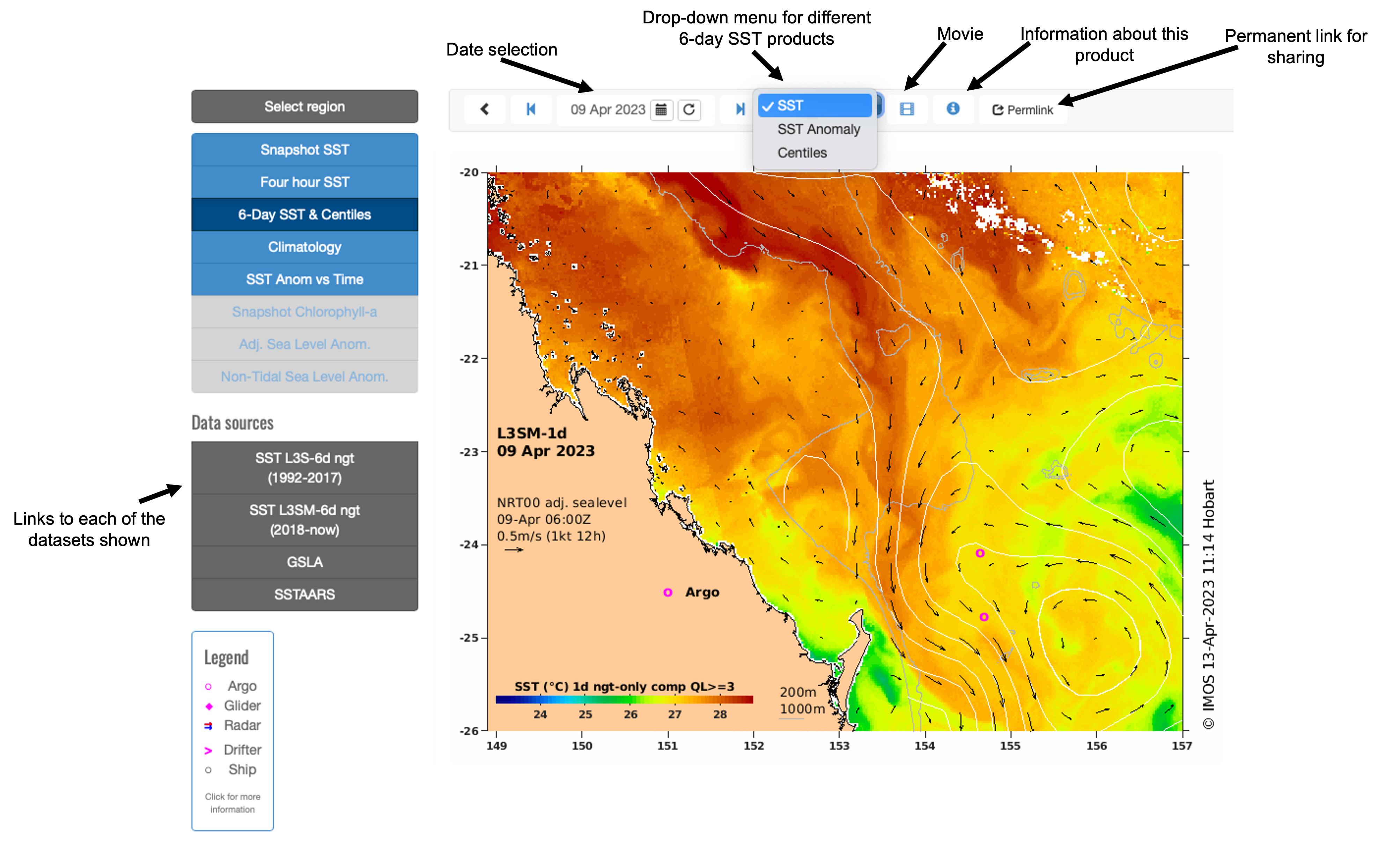
We have several ways of looking at local regions: Snapshot maps of Sea Surface Temperature (SST), 4-hour composites of SST, 6-day composites of SST, MyOceanCurrent, and Google Earth (Figure 1).
With one exception, satellite-borne sensors that measure SST remotely cannot see through clouds. We have different ways to deal with the occurrence of clouds in a region. In the Snapshot SST product, we overplot newest data on top of older data, to fill the cloud gaps without doing temporal averaging in cloud-free regions. In the 4-hour and 6-day SST products, we create time-averaged composites using data from several different satellites over those time windows.
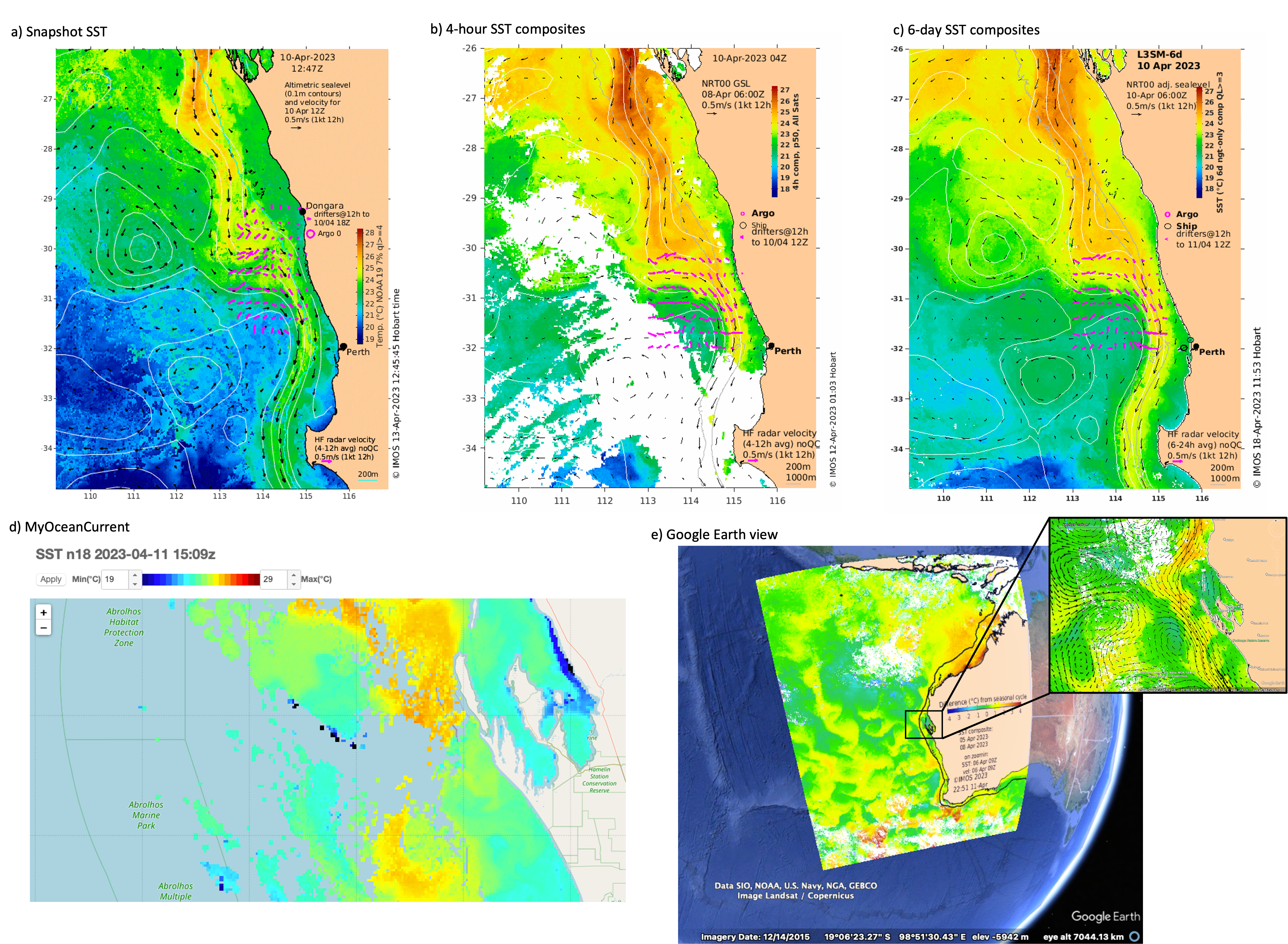
Snapshot SST and 4-hour SST
In the Snapshot SST product (e.g., Figure 1a), for every overpass of a polar orbiting satellite that measures SST, we make a new map (from a single IMOS L3U data file). This map is the previous map updated only where there is data of good quality in clear-sky regions. If those clear-sky regions are large and last for several satellite overpasses, animation of the imagery shows the complex patterns of movement clearly. Where the clear-sky regions are small and transient, however, this process leads to a messy patchwork of little value. View the animation several times and you will see the varying quality and usefulness of the images as the weather swings between clear and cloudy.
The colourbar of the Snapshot SST maps (Figure 1a), apart from showing the temperature scale, lists the name of the satellite that measured that region at that time and the fraction of the scene with new data of acceptable quality. The leading cause of data gaps is cloud cover, and poor data quality is mostly due to contamination by thin or patchy clouds. Bear this in mind as you step through images, which is most quickly done using the animations.
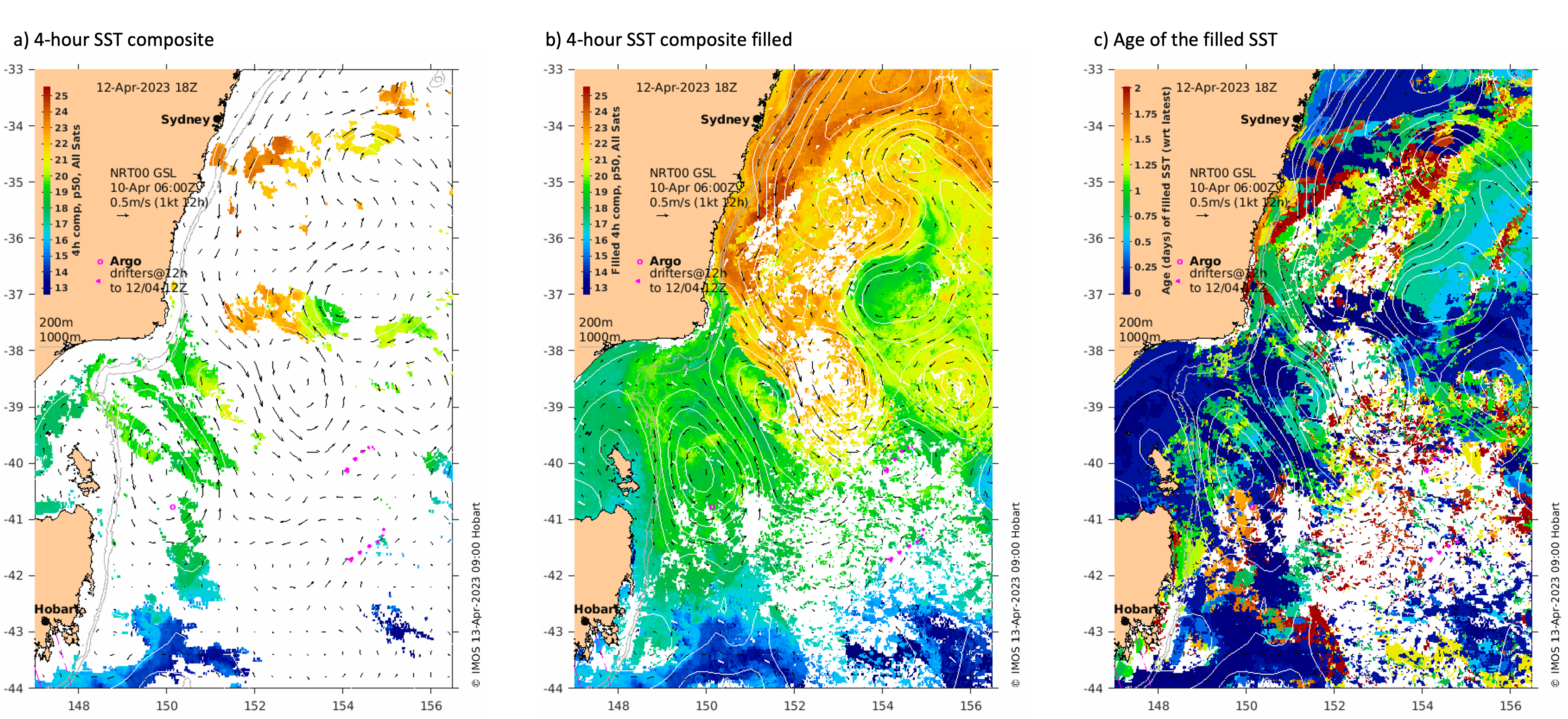
The 4-hour SST composites use all available SST sensed by the satellites in orbit over the past 4 hours - including data from the (relatively) new Japanese geostationary Himawari satellites, which acquire an image every 10 minutes. To build a composite, we average all the data available for each grid cell of a 2 km × 2 km grid. If too many grid cells have no data available over that period, likely because of clouds, the maps are quite empty of information (e.g., Figure 2a). For that reason, we also provide a 'Filled 4-hour SST' product, where the blank grid cells are filled with previous 4-hour composites (Figure 2b). You can then assess if this filled product is relevant to you by looking at the 'Age' map, which shows how many days ago the data shown in each grid cell was observed (Figure 2c). Some ocean features form and dissipate quickly, especially in near-coastal regions. For these, SST data from 2 days ago might not be useful anymore.
Something to consider is that day-time satellite passes, especially in warmer regions, are often affected by a 'warm skin' effect. This effect occurs if there is very little wind, allowing the uppermost few centimetres of the ocean to become several degrees warmer than immediately below. A warm-skin-affected image shows an accurate measurement of sea surface temperature, but it is not very useful for visualizing the ocean currents. For this reason, we also included wind maps in the drop-down menu of the 4-hour SST product — here's an example of the wind field off the Torres Strait.
We also provide 1-day composite images of SST anomaly in .kml files to be opened in Google Earth (Figure 1e). When using Google Earth, you can zoom in the regions of interest. The anomaly is shown to enhance detail without the colourbar changing as you zoom and pan. These files also include altimeter-derived estimates of currents. Some patience is required to use this product, because many images have to be loaded into Google Earth, especially if you zoom right in. Note that the time slider allows you to change the date. You may have your own Google Earth viewable data, e.g. trajectories of objects, that you can overlay on the SST imagery.
6-day SST composites, SST anomalies, and SST centiles
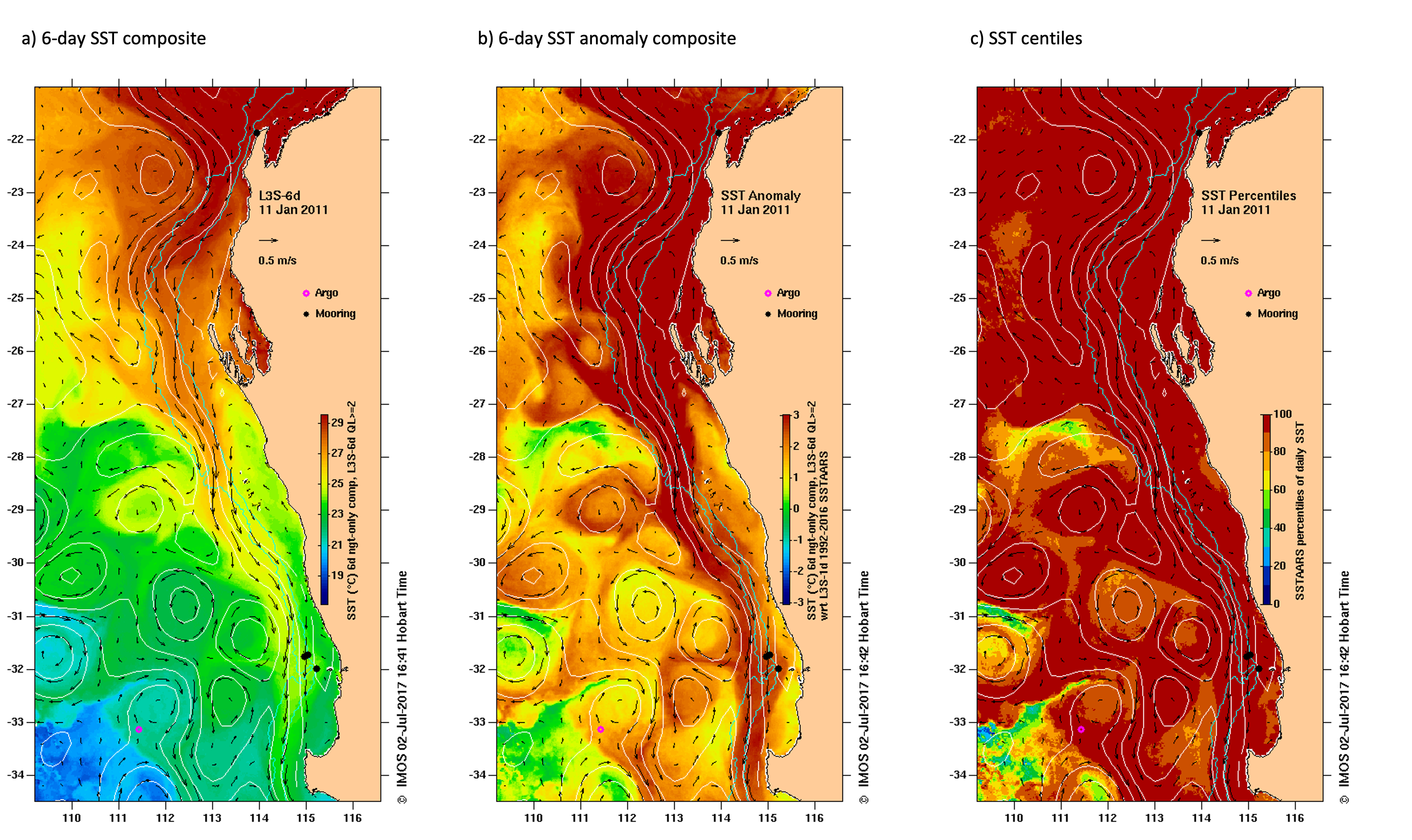
The 6-day SST composites (e.g., Figure 3a) show multi-sensor composite data produced by the Bureau of Meteorology, using GHRSST protocol. These composites include only night-time data, to minimise bias due to diurnal heating. To access these maps click on the 'Sea Surface Temperature' map in the carousel on the frontpage, and then select your region.
You can look at the 6-day SST anomaly maps (Figure 3b) to see how the SST values differ from what is normal for that time of the year. These anomalies are calculated relative to the SST Atlas of Australian Regional Seas (SSTAARS) climatology (1992-2016). For this analysis, the SST trend is not removed. To access these maps click on the drop down menu at the top of the 6-day SST map of your selected region.
The 6-day SST anomaly centile maps (Figure 3c) shows in which centile the SST anomaly of each pixel falls within 25 years of anomalies (1992-2016). The percentiles have been evaluated at each pixel for every day of the year. Anomalies falling in the <10 rank (dark blue) are the coldest 10% of observed anomalies at that pixel for that day of the year. Similarly, anomalies ranked >90 (red) are the hottest 10% of observed anomalies. Green percentiles represent the average 20% of temperature anomalies. Therefore, if you are interested in looking at an extreme SST heating or cooling event, you can refer to these maps to check how extreme was that event for that region at that time of the year. To access these maps click on the drop down menu at the top of the 6-day SST map of your selected region.
Figure 3 shows the 6-day composites for SST, SST anomaly, and SST anomaly centiles off Western Australia's coast during the 2010/2011 marine heatwave. At that time, most of the ocean's SST exceeded the 90th centile for several weeks, having a large impact on the ecosystem of that region.
Datasets integration: SST, sea level data, and in-situ data
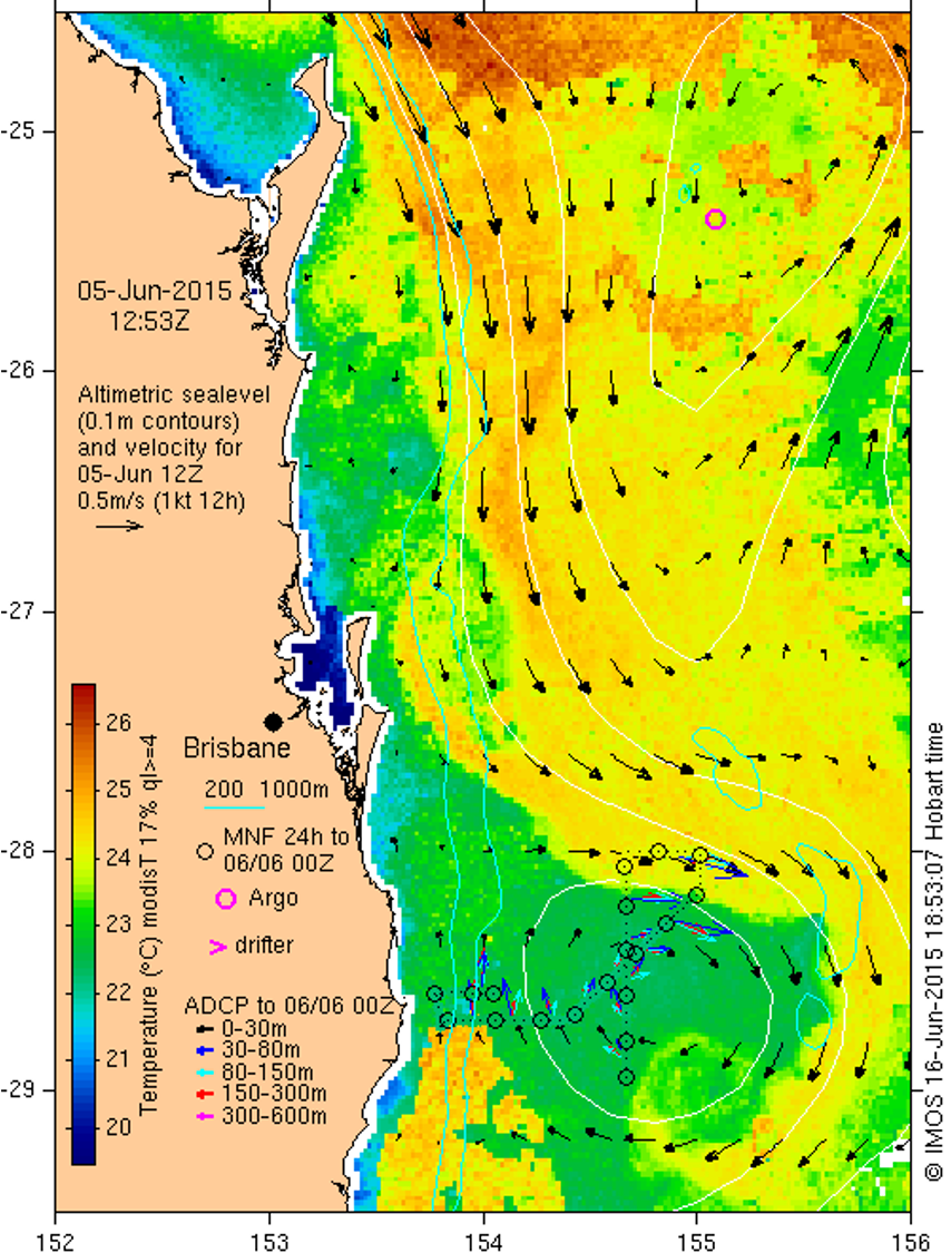
Overlaid on the temperature imagery is several other data, including the adjusted sea level anomalies (contours at 0.1 m, read more below), the geostrophic current velocity field derived from gradients of sea level, and the more localised data from high-frequency radars, ships, Argo floats, gliders, current meters, and surface drifters, as detailed in the legend for each of the maps. You can click on the Argo floats (magenta circles popping up at different locations each day) to see the profiles of temperature and salinity measured by them at that location. During some oceanographic campaigns, we have a beautiful collection of data complementing the SST maps, as was the case for the super-star 'Freddy' (frontal-eddy), during an RV Investigator cruise in June 2015 (Figure 4).
Velocity estimates from the various sources are shown in one of three ways. Straight arrows are used for current meters and gliders. Curved arrows are used for high-frequency radar and altimetry. The scaling is the same for both arrow types, The difference is that the curved arrows use the 2-dimensional information of the gridded velocity types, by integrating Lagrangian trajectories. For both arrow types, the scaling has dimensions of time (screen distance per velocity unit), which can be interpreted as how far a particle will drift over a certain interval of time. For zoomed-in maps of high-current regions we use short (e.g. 3 or 6h) times to avoid over-crowding of arrows while for weak current regions we use longer times (e.g. 12 or 24h) as shown in the velocity key.
The interval between map times is determined by the SST imagery and is not uniform, or synchronised with the other data. The adj. SLA information is a few days older than the latest temperature image, because it takes many days for the altimeters, to sample the globe. The maps are replotted daily until these two data types become contemporaneous. Other data are available at ranges of times as indicated.
MyOceanCurrent
In the MyOceanCurrent section of the website (e.g., Figure 1d), you can zoom into your region of interest to look at the latest SST data. Here, you'll be able to see finer scale SST features. This dataset is affected by cloud coverage, because each map only shows data measured by one satellite, instead of a composite of data from several satellites as in the previous products. If you click on this product's 'help' button you'll see all the functionality available, including saving your favourite regions for recurrent viewing, and choosing a viewing option optimized for low-bandwidth internet connections. Another difference between the MyOceanCurrent maps and the other SST products is that in MyOceanCurrent you'll only see the most up-to-date data available, but no historical maps are stored.
Which SST map should you look at? That depends on your goal.
For sea-going activities, Snapshot and the 4-hour SST maps are probably most useful. Vessels such as RV Investigator upload their sampling data, so the ship's position and ship-board SST measurements appear on our website in near-real time. Here, is an example of SST measurements taken by the RV Investigator during a voyage in 2023, on a very cloudy day in Tasmania.
If you are in a region of low-bandwidth internet, like the middle of the ocean, we suggest creating a login in MyOceanCurrent. Then, you'll be able to personalise the SST maps to your area of interest and access it easily.
For an analysis over a long time period, we suggest watching the 6-day SST and SST anomaly movies, and then checking the daily map to look at additional data sources, like gliders, Argo floats, drifters, ship-board measurements, current meters, and even CTDs carried by seals.
For studies of extreme ocean conditions, we suggest using the SST centile and Adj. SLA centile products. The first product will give you information on how patterns of extreme SST are changing over time, and where warming hotspots are emerging. The second product will give insights if the water column in a specific region has been warming as a whole, and hence increasing the thermosteric height of the ocean. You can also look at sub-surface temperatures measured by sensor attached to Argo floats and seals in your region of interest. And you can check how the SST over a local region has been changing in time in these bar plots of SST anomaly (example for the region off NSW).
State Regions
State Regions are available in two different time scales:
- Monthly means of SST and Adjusted Sea Level Anomalies (Adj. SLA)
- 6-day SST composites, anomalies, and centiles, described above. You can also see Adj. SLA and 6-day SST maps side-by-side (Figure 5).
Adjusted Sea Level and Adjusted Sea Level Anomaly maps
Adjusted Sea Level is the sea level minus two rapidly-varying sea level signals mostly due to barotropic dynamics: astronomical tides and the ocean's response to atmospheric pressure (which is to rise about 10 cm for each 10 hPa fall of pressure). Adjusted Sea Level is thus a measure of the slow modes of the ocean. The slow modes are largely in geostrophic balance, so we can estimate the near-surface velocity from the gradients of Adjusted Sea Level. Adjusted Sea Level is also a measure of depth-integrated density (and thus ocean heat content), as shown on our Argo floats where Adjusted Sea Level is compared with in-situ determinations of steric height anomaly.
We used to call the Adjusted Sea Level 'Gridded Sea Level', but changed the name in September 2021. The once-traditional term 'adjusted' is commonly omitted by many agencies and oceanographers. We did this, too, then regretted it, because dropping the 'adjusted' leaves no short name for 'unadjusted sea level', which is the quantity most relevant to users interested in coastal inundation (see our Australia/NZ maps of Non-Tidal Sea Level). Another candidate name for Adjusted Sea Level is ocean dynamic sea level. Related names include: dynamic height, dynamic topography, and subsurface pressure.
The Adjusted Sea Level Anomaly (Adj. SLA) is the form in which altimeter data is most often used, and indeed some users simply call this 'altimetric sea level', or 'sea surface height' or similar, without being clear that it is adjusted, and the anomaly.
'Adjusted' means that sea level variations due to high-frequency processes have been subtracted from the observations. These high-frequency processes are the fast (predominately barotropic) modes of the ocean: the ocean tides and the ocean's short-term response to atmospheric pressure and wind stress. With these high-frequency signals subtracted, the remaining signals are due to lower-frequency dynamics, i.e. the slow modes of the ocean (which are predominately baroclinic). Altimeter data is sufficiently frequent to adequately sample the slow modes, but not the fast modes.
'Anomaly' is the departure from the long-term (1993-2018) mean. To understand why we use the anomaly, one has to understand that the shape of the ocean's surface is mainly (by a factor of about 100) a product of small perturbations of the gravity field, not ocean dynamics. Altimeters have been measuring the surface of the ocean precisely since 1992. The time-mean of all those measurements is called the Mean Sea Surface (MSS). 99% of that is due to gravity perturbations and is called the geoid. The problem is that the geoid is not independently known with sufficient accuracy that it can be simply subtracted from the altimeter observations in order to do oceanography using the residual. Instead, we subtract the MSS and accept that, in so doing, we are also removing the steady part of the signal due to the ocean (the so-called Mean Dynamic Topography, or MDT), leaving just the anomaly (or transient part).
In Figure 5 (left), for example, the Adj. SLA field is a map of tidal-residual, isostatically-adjusted sea level anomaly, valid for the analysis date T_a shown, which is normally five days ago. The atmospheric pressure map (blue contours are lows, white contours are high) used for making the isostatic adjustment is shown because features of the circulation (e.g. near the coast, or under a tropical cyclone) can sometimes be explained by the winds.
How do we know that the ocean has areas where the water is raised or lowered by half a meter or so, for 100's of km? If you look closely, you will see lines of little white, magenta or black dots. These lines show where satellites carrying radar altimeters, have flown over, measuring the distance from the satellite down to the water. That distance is a little shorter where the sea level is raised a bit. The fact that that difference can be accurately measured is a great triumph of engineering, and is one of the key breakthroughs responsible for the present revolution in ocean observation. The colour of the dot indicates when the satellite flew over. White means more recently than T_a, magenta means the three days previous, black means longer ago.
The bar plot in Figure 5 (left) lists the satellites flying altimetry missions that were used to calculate the Adj. SLA shown in the map. This bar plot shows the history, from 7 days before, to 3 days after T_a, of the daily number of observations made by each of the satellites, within the region shown. (More precisely, each sea level 'observation' is a 2 km-wide average along 25 km of the flight path). The satellites can't sample the whole world every day because these types of altimeters can only measure directly beneath them. To make a complete 'quasi-synoptic' map, we must therefore use data that is up to 10 days old. This is OK for tracking the movement of 'mesoscale' (∼100km or greater) features like ocean eddies, but not the small features sometimes trackable in sequences of SST images. The older data points are down-weighted compared to the newer ones in making the map. Where there is only old data or no data at all, the estimated anomaly relaxes to zero and the map is obviously least useful.
The other (and much older) way of measuring sea level is by tide gauge. Australia has many of these in ports all around the country. We include these data in our maps by averaging-out the tides and making the same atmospheric pressure correction as with the altimeter estimates, then interpolating the results at many points along the coastline between the gauges. This is the key difference between our maps and global maps available from international sources. Both the observed and interpolated coastal observations are shown on the map. Coastal sea level changes more rapidly than deep-ocean sea level, so it is just as well that the coastal observations are made much more frequently than those by satellite over the deep sea. The resulting estimates of along-shore geostrophic current are not always accurate, but are at least indicative of a shelf-wide average flow.
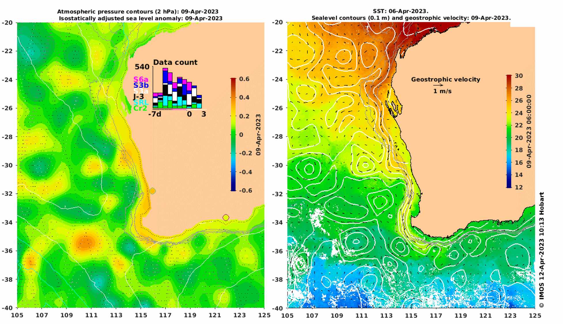
SST and Adjusted Sea Level maps, side-by-side
The colour-coded field on the right of Figure 5 is a map of Sea Surface Temperature (SST) which is formed by compositing single images over a 6-day period, in order to obtain a relatively cloud-free map without averaging-out useful detail. This is the same 6-day SST composite product described in the section above, and accessible via the carousel on the frontpage. This latter version has overlain data from high-frequency radars, ships, Argo floats, gliders, current meters, and surface drifters.
Maps of SST show the Adjusted Sea Level map again (Figure 5, right), but this time as total Adjusted Sea Level, i.e., the anomaly plus a model-based estimate of the mean dynamic topography (see above). Being overlain on SST, the Adjusted Sea Level is shown just as white contour lines. The result is the oceanographer's weather-map, with sea level taking the place of air pressure, and ocean current taking the place of the wind. The physics associated with the Earth's rotation is analogous to weather systems: geostrophic currents run with the high on their left in the southern hemisphere. Black arrow heads depict the direction and strength of the ocean currents. Reference should be made to the distribution (left panel) of the available data in order to judge the reliability of these estimates. Where no recent data are available, this map will show our estimate of the time-mean sea level slopes and currents (the reliability of which also varies regionally depending on numerous factors).
The SST map is best for precisely locating where the ocean currents are, while the sea level map is good for resolving ambiguities of which way the currents are generally flowing, and whether they are weak or strong. The accuracy of both maps is instructively judged by comparing them with the trajectories and speeds of Global Drifter Program drifters, which are shown in magenta in the SST maps. Drifters sometimes travel at up to twice the speed that we estimate from the sea level maps because they measure the velocity at a point, while the map shows the average velocity over many kilometres and a period of days.
Please note: neither the satellite nor the coastal sea level near-real-time data streams are fully quality-controlled, and errors do occur.
If you click on the Data Sources, listed on the left of each map (Figure 6), you'll be directed to the Australian Ocean Data Network (AODN) portal, where you can subset and download the data you are interested in.
Australian Region
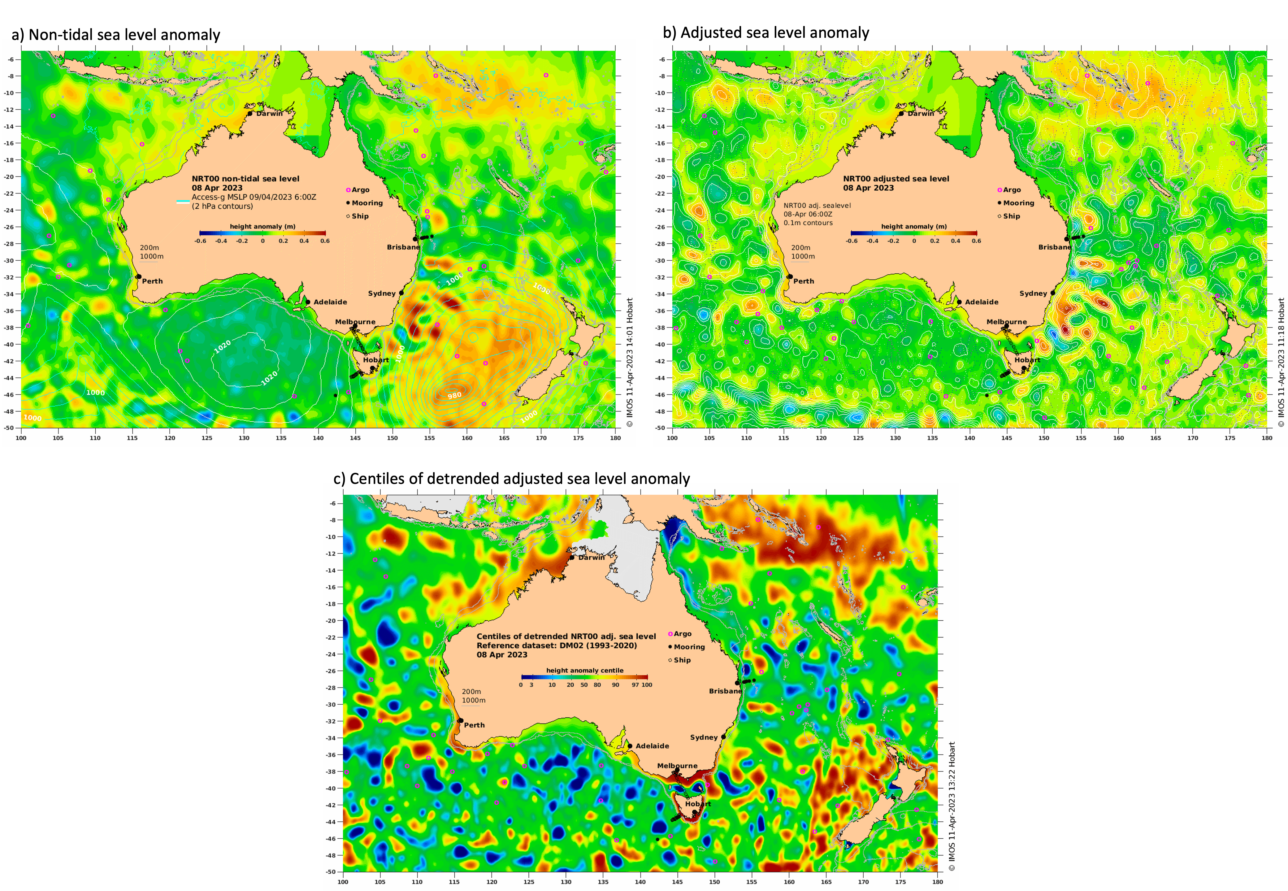
Maps of the whole Australian Region show 6-day composites of SST, and several flavours of Sea Level Anomaly (Figure 7): Adj. SLA, Adj. SLA centiles, and Non-Tidal SLA (select your flavour on the dropdown menu and left-side menu of each daily map).
The Adj. SLA maps (Figure 7b) show the isostatically adjusted sea level anomaly with the data used in its estimation overlaid (dotted lines). For more information on what's show in this map, refer to the text above, in the 'Adjusted Sea Level and Adjusted Sea Level Anomaly maps' section. You can also see a map of adj. SLA over a larger region, extending to the Kerguelen Plateau in the southern Indian Ocean here. In this larger region, we also plot isolines of atmospheric pressure (blue and white contours).
Centile rankings of (daily, detrended) Adjusted Sea Level Anomaly
In the Adj. SLA maps we often see patterns of strong positive or negative anomalies. However, it is difficult to know if that pattern is extreme or if it is just a common oceanographic feature in that region. To answer that, you can look at the maps of Adj. SLA centiles (Figure 7c). These maps are a way of seeing “how anomalous” the anomaly at a particular place and time is, compared with past anomalies at the same place. But sea level anomalies are not randomly distributed about a mean value, because sea level has a significant trend; about 100 mm in the last 28 years (∼3.7 mm/year). Nor does it have a very regular annual cycle (see time series plot of the Australasia-region average adjusted sea level anomaly). So we have chosen to show the daily centile rankings of Adj. SLA after subtracting the Australasia-region trend, but not the average annual cycle, in contrast to how we rank anomalies of Sea Surface Temperature. Otherwise, the interpretation of the centile maps is the same: if a point on the map is red, it means that the adjusted sea level that day, at that location, falls within the top few percent of all observed anomalies (detrended as described above). Note that we have used a non-linear colour scale, in order to show more discrimination at the high and low ends.
The centile levels of the 28-year, detrended data set found here, is the reference data set against which the detrended anomalies for a particular day are compared. For efficiency, it is not re-computed every day. Consequently, and because eddies do not follow in each other's tracks, new observations can fall outside the range of the centile levels of the reference data set.
Non-Tidal Sea Level and Non-tidal Sea Level Anomaly
For this large Australian region we also include a map of sea level that includes the sea level anomalies observed by satellites with addition of wind and pressure-driven changes of sea level as well as many other (non-tidal) causes of variation such as El Niño and ocean eddies. We call this Non-Tidal Sea Level Anomaly (Non-Tidal SLA; Figure 7a). The Non-Tidal SLA is sometimes referred to as either 'tidal residual' or 'non-tidal residual'. Both (confusingly) refer to the signal left over once a tidal prediction or analysis, which usually includes the mean, is subtracted.
Our maps of Non-Tidal SLA do not include some of the processes that can be important in shallow (<∼30m) areas, nearshore (<1km) areas, or over short (<12h) time intervals, such as wave setup, seiches or tsunamis. For this reason, we only show Non-Tidal SLA for the Australia-wide maps.
It is not possible to make maps of Non-Tidal SLA directly from altimeter observations because non-tidal SLA changes so rapidly compared to altimetry coverage. So OceanCurrent's maps of Non-Tidal SLA are made by adding the 'static' Inverted Barometer response at 6h intervals to our daily maps of Adj. Sea Level Anomaly made from a combination of altimeter and coastal tide gauge observations of adjusted sea level anomaly. The static inverse barometer is a fairly good approximation of the transient inverse barometer response, and is P'/(ρg) where P' is atmospheric pressure minus the daily, global over-ocean mean, ρ is the average density of sea water and g is gravity. You can see how quickly the atmospheric conditions change, and how those changes affect the ocean, when you watch the Non-Tidal SLA movies.
How to compare all these sea level maps?
Figure 6 shows all the available sea level maps for the large Australia region. At the day of analysis, the Tasman Sea and the tropical western Pacific had high values of Non-Tidal SLA (>0.3 m, Figure 7a). The map of Adj. SLA for the same date (Figure 7b), still shows high values in the tropical western Pacific, but the strong signal in the Tasman Sea is now scattered into smaller mesoscale features off New South Wales, and a positive 'blob' off the west coast of New Zealand. The absence of the wide-spread high values in the Adj. SLA map indicates that whatever was causing those high values in the Non-Tidal SLA was removed (or, adjusted). If you look back at the Non-Tidal SLA map, you'll see an atmospheric low-pressure system located half-way between Tasmania and New Zealand's South Island (see the cyan contours decreasing from 980 hPa at ∼170°E, 46°S). That low pressure system means that there is less weight of the atmosphere acting on the ocean's free surface and, therefore, this surface is able to rise above its mean state. Conversely, an atmospheric high pressure system pushes the ocean's free surface towards the ocean's interior, and is seen as negative Non-Tidal SLA, as it often occurs south of the Great Australian Bight.
With the effect of the atmosphere (and other non-tidal variations) removed, we now know that for the day of analysis in Figure 7, the high Adj. SLA seen off NSW and off NZ's west coast are caused by ocean conditions only. Off NSW, the alternating positive and negative Adj. SLA indicate the presence of a train of eddies that slowly move southward. Off NZ, however, there is no strong ocean circulation that could be responsible for this regional high Adj. SLA. Looking at the Adj. SLA centile map (Figure 7c), the values we see off NZ fall within the higher end of the distribution (97-100th centile). What could be causing these anomalously high Adj. SLA off NZ? This requires a new investigation, but persistently hot waters in that region over the previous summer could be an answer.
Some explanation of oceanographic terminology, techniques, and principles
- Altimeter
-
 A satellite altimeter measures the range from the satellite to the sea surface directly below using a very
precise radar. The orbital position of the satellite is also known very precisely because altimetry satellites
use a combination of GPS, DORIS and laser ranging to carefully monitor the orbit of the satellite. The
difference of the range and the orbit is the height (averaged over space - the 2km-radius footprint of the
radar, and time - 1Hz averages are about 7km apart) of the sea surface (effectively relative to the center of
the Earth). Amazingly, the sea surface height can be determined to centimeter accuracy, once a
number of corrections are made, e.g. for the wet troposphere path delay, the sea-state bias and the instrumental
bias.
More information:
A satellite altimeter measures the range from the satellite to the sea surface directly below using a very
precise radar. The orbital position of the satellite is also known very precisely because altimetry satellites
use a combination of GPS, DORIS and laser ranging to carefully monitor the orbit of the satellite. The
difference of the range and the orbit is the height (averaged over space - the 2km-radius footprint of the
radar, and time - 1Hz averages are about 7km apart) of the sea surface (effectively relative to the center of
the Earth). Amazingly, the sea surface height can be determined to centimeter accuracy, once a
number of corrections are made, e.g. for the wet troposphere path delay, the sea-state bias and the instrumental
bias.
More information:
Ocean Surface Topography at NASA JPL
Satellite Altimetry at AVISO
Broadview Radar Altimetry Tutorial (BRAT) - AVHRR
- Advanced Very High Resolution Radiometer. A sensor carried by the US National Ocean and Atmosphere Administration (NOAA) satellites which oceanographers use to measure Sea Surface Temperature (SST). The pixel size is about 1km and accuracy about +/-0.6°C. The NOAA satellites broadcast the data continuously, so any groundstation that can see the satellite can receive the data. Several satellite passes per day are tracked, received, processed and archived at WASTAC in Perth, Bureau of Meteorology in Melbourne, CSIRO in Hobart and ACRES in Alice Springs.
- CARS - the CSIRO Atlas of Regional Seas
- The name is no longer very appropriate, since the CARS2009 version of this season-resolving hydrographic atlas covers the entire globe. It is produced by interpolating all available in-situ observations of hydrographic properties onto a regular three-dimensional grid. The result is a set of harmonic constants for the yearly and semi-annual components of the variability as well as the all-time mean. The sudden increase in the amount of data provided by the Argo programme means that the atlas is not really a long-term average so it is best to interpret it as simply an average of all available data, binned by time-of-year, but not year itself.
- Coastal Trapped Wave
- Otherwise known as a topographic Rossby Wave, a Coastal Trapped Wave (CTW) is a large-scale, sub-inertial wave with the striking property of only propagating along the continental margin, rather than in whatever direction it is forced. In the southern hemisphere, a CTW propagates with the coast on its left. CTWs generated by cyclones off the north-west shelf can be tracked all the way to Victoria. CTWs generated in the Great Australian Bight have an effect at Sydney. Real-world CTWs have properties in common with two sorts of idealised waves. The propagation speed of (barotropic) Continental Shelf Waves depends on the width and slope of the continental margin, while (baroclinic) Internal Kelvin Waves propagate along vertical (by definition) boundaries in the presence of stratification. Thus, the phase (and group) speed of the CTW is determined by the shape of the shelf and the strength of the stratification, and ranges from 10m/s (e.g. where the shelf is very wide) to 1m/s or even less in some places. Pulses of current, sometimes up to 0.5m/s, accompany the sea level signal and there is also an effect on the depth of the thermocline that mirrors the sea level signal. Harmonic solutions (i.e. periodic in time) of the CTW equations comprise a number of discrete wavenumbers for each frequency. High mode-number solutions have progressively shorter along-shelf wavelengths (and therefore lower phase speed) and progressively more antinodes in the across-shelf amplitudes of sea level, velocity and thermocline displacement.
- Coriolis force
- The `pseudo-force' on an object moving with respect to a rotating frame of reference. A cannon shell appears to veer left in the southern hemisphere, and right in the northern hemisphere.
- Ekman velocity
- A steady wind blowing over the open ocean causes the surface layer of water to move at a velocity (called the 'Ekman velocity') which is such that the Coriolis force on the layer balances the force of the wind. Hence, a wind from the south drives an Ekman velocity towards the west, in the southern hemisphere. The thickness of this layer is variable, with 30-50m being fairly typical. The Ekman velocity is additional to whatever velocity the surface layer was moving at before the wind commenced, and takes a day or two to settle down to being at right angles to the wind. The oscillations that follow a sudden change of the wind stress are called inertial oscillations.
- Gridded (Adjusted) Sea Level Anomaly
- This is the name used on this website for the gridded maps of Adjusted Sea Level Anomaly that we make by combining the data from many altimeters and tide gauges. Read more about these maps in the Adj. SL and Adj. SLA section. Being a two-dimensional map, it is possible to use the very simple and surprisingly-accurate geostrophic equations to determine the surface velocity field associated with the surface pressure gradient caused by the gradient of GSLA (as distinct, for example, from the Ekman velocity and the Stokes drift). Most of the graphics, however, show the velocity field determined from Gridded (Adjusted) Sea Level. You can download these daily maps of GSLA and surface geostrophic velocity in both Near-Real Time and Delayed Mode from the AODN website (or here, for the thredds server).
- Gridded (Adjusted) Sea Level
- Gridded (Adjusted) Sea Level (GSL) is the name we use for our estimate of the Dynamic Topography obtained by adding the CAST2008 Mean Dynamic Topography to Gridded Sea Level Anomaly (GSLA). Geostrophic currents computed from GSL include the time-mean and are therefore much more directly comparable with in-situ measurements of surface current velocity such as those determined from the trajectories of surface drifters. Why do we need to use CAST2008? While the geoid remains unknown with sufficient spatial resolution, the only way to remove the influence of the geoid from altimetric measurements of the Sea Surface Height is to subtract the long-term-mean of the observations, which, unfortunately, also subtracts the time-mean component of the Dynamic Topography. Read more about these maps in the Adj. SL and Adj. SLA section. The GSL maps are contained in the GSLA and surface geostrophic velocity files described in the Gridded (Adjusted)SLA and available in both Near-Real Time and Delayed Mode from the AODN website (or here, for the thredds server).
- Geostrophic Balance
- Balance between the pressure gradient and the Coriolis force. In the southern hemisphere, a northward current is geostrophically balanced by sea level slope rising to the west. Similarly, an anti-clockwise rotating body of water, or 'eddy' has elevated sea level in the centre. Slowly-varying (ie, over several days and over 'large', e.g. 50km or more, distances) currents are invariably close to being geostrophic, so by measuring either the current velocity or the slope of sea level, the other can be calculated. The same principle applies in meteorology: the wind blows anticlockwise around a high pressure system in the southern hemisphere, and clockwise around a low, or cyclonic, system. More rapidly-varying (in time or space) sea level slopes are much less likely to be geostrophic, so estimation of velocity from sea level requires many other factors to be taken into account, such as the wind stress, curvature of the sea level gradients, etc.
- Geoid
- The surface to which the ocean would conform if all the ocean currents came to rest. It is a very irregular surface, with highs and lows of 30m or more that mirror the small-scale and large-scale irregularities of the Earth's gravity, due, for example, to variations of the depth of the ocean. The difference between the Mean Sea Surface (MSS) and the geoid is called the Mean Dynamic Topography.
- Inverse barometer
- To a fairly good approximation, a local reduction of atmospheric pressure of 10hPa leads to a sea level rise of 10cm. This rise of sea level will be recorded by tidegauges and satellites but needs to be removed in order to monitor the internal dynamics of the ocean, because the important quantity is the total pressure just below the ocean surface, which is the atmospheric pressure plus the hydrostatic pressure due to any local elevation of the sea surface.
- Isostatic Adjustment
- When we refer to 'isostatically-adjusted' sea level, we mean we have subtracted the 'inverse barometer' response of sea level to fluctuations of local atmospheric pressure.
- Sea Level Anomaly
- See a detailed explanation in the Adjusted Sea Level and Adjusted Sea Level Anomaly section.
- Sea Surface Height
- The spatial structure of the Sea Surface Height is mostly due to the undulations of the geoid. Only a small part of the variability is due to the mean and time-varying components of the 'dynamic topography' associated with ocean circulation. The shape of the geoid is not known precisely, but we can assume that it does not vary much with time. The average over time of the altimetric sea surface height (the Mean Sea Surface) is the sum of the geoid and the mean dynamic topography. By subtracting the mean sea surface from altimeter measurements of the Sea Surface Height we are therefore left with the variable part of the dynamic topography. From this we subtract model estimates of the high frequency signals due to tides and the inverse barometer effect, leaving an estimate of the Adjusted Sea Level Anomaly which can be used to map the time-varying part of the highs and lows of the ocean surface around which the transient component of geostrophic currents flow.
- Sea Surface Temperature
- Usually measured either continuously from ship at the depth of the engine water intake, or remotely by satellite (see AVHRR) or airplane.
- SynTS
- Short for 'synthetic temperature and salinity', as explained at [what's shown]. The synTS method is described by Ridgway and Dunn (2010).
- Surface Drifter
- The principle method for validating our altimetric surface velocity estimates is by comparing them to the velocity of Surface Drifters, or Global Lagrangian Drifters. These buoys are tracked by the Argos positioning system (not to be confused with the Argo floats) and have a 10m long sea-anchor at the end of a 10m wire, to minimise their down-wind velocity, thus reducing their sensitivity to those components of the surface current velocity to which the altimeters are blind.
- Upwelling
- When water is drawn to the surface from great depth. It is a very significant phenomenon because it makes nutrients that have settled to depth become available again to phytoplankton living within the depth of penetration of sunlight. Various forces drive upwelling. At the coast, alongshore winds that have the coast on their right in the southern hemisphere drive the surface waters away from the coast in the Ekman layer. That water has to be replaced, so it rises from below. The place where this happens most strongly in Australia is known as the Bonney Coast, between Portland and Robe.
- Wind Stress
- The effect on the ocean of the wind increases greatly as the wind velocity increases. The wind stress is a measure of this effect and is approximately proportional to the square of the wind velocity.